To avoid enemy radar detection, modern fighters, ships and missiles should have the smallest effective scattering area (EPR). Scientists and engineers who develop such barely visible objects, using computational electrodynamics techniques, optimize the EPR and the effects of scattering of arbitrary objects when using radars. The object in question scatters electromagnetic waves incident on it in all directions, and part of the energy returned to the source of electromagnetic waves in the process of so-called. backscattering, forms a kind of "echo" of the object. EPR is just a measure of the intensity of the radar echo.

In practice, a reference conducting sphere is used as an object for radar calibration. A similar formulation of the problem is used to verify the EPR numerical calculation, since the solution of this classical problem of electrodynamics was obtained by Gustav Mie in 1908 .

In this note, we will describe how to carry out such a standard calculation using an effective two-dimensional axisymmetric formulation, and also briefly note the general principles for solving a wide class of scattering problems in COMSOL Multiphysics ^® .

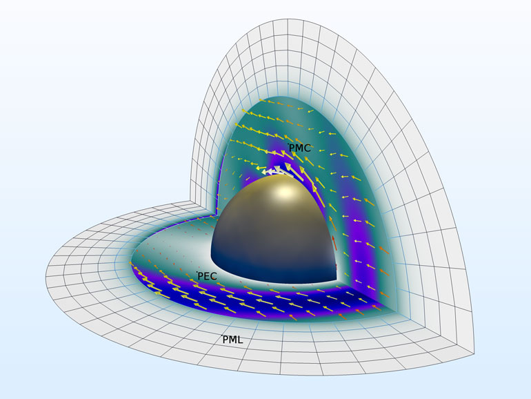
Fig.1. The distribution of the electric field (its norm) and the time-averaged energy flow (arrows) around an ideally conducting sphere in free space.

Scattering on a conducting sphere: size matters

In the classical reference example , an ideally conducting metal sphere in free space is irradiated with a plane electromagnetic wave and the EPR is calculated.

The output is usually calculated scattering in for different ratios of the sphere radius and wavelength, on the basis of which there are three areas: Rayleigh , optical and transition Mi-range.

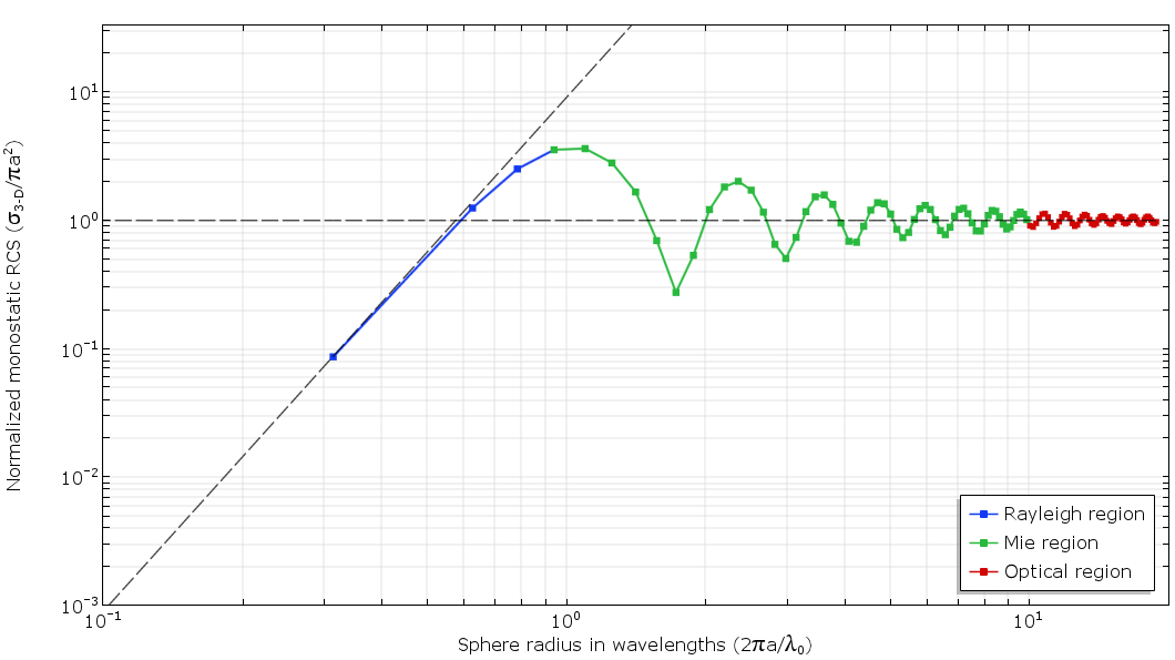
Fig. 2. Graph of EPR versus wavelength (in double logarithmic scale). Three characteristic regions were identified: Rayleigh, Mi, and optical. Black dashed lines indicate asymptotic solutions for the Rayleigh and optical zones.

The EPR characteristics are significantly influenced by the electrical size and material properties of the object on which the radar beam falls. Since the electrical size of the object — in our case, the sphere — decreases when going from the optical range to the Rayleigh region (via the MI range), asymptotic methods will not provide sufficient accuracy to take into account the contribution of all physical phenomena. To obtain accurate results, the problem should be solved with the help of full-wave techniques .

In the three-dimensional formulation, even taking into account the use of perfectly matched layers (Perfectly Matched Layers - PML), which effectively restrict the computational domain and simulate open boundaries, and symmetry conditions, the calculation with detailed frequency / wavelength resolution can take quite a long time.

Setting symmetry conditions for electrodynamic calculations

Подробнее тут.

Fortunately, if the object is axisymmetric and scatters waves isotropically, a full 3d analysis is not required. To analyze the propagation of electromagnetic waves and the resonant behavior of an object, it suffices to carry out a calculation for its cross section in a two-dimensional axisymmetric formulation when specifying certain conditions.

Two-dimensional axisymmetric model of the microwave process: a view from the inside

Suppose that our sphere is metallic and has high conductivity. For this task, the surface of the sphere is defined as an ideal electrical conductor (PEC), and its inner part is excluded from the computational domain. The area around it is defined as a vacuum with the corresponding material properties, and in the outermost layer is used PML spherical type, used to absorb all outgoing waves and prevent reflection from the boundaries of the computational region.

Modeling of metal objects in wave electromagnetic problems

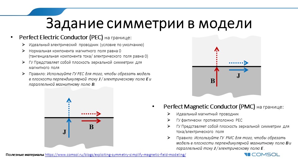
Для численного решения задач электродинамики в частотной области существует несколько приемов для эффективного моделирования металлических объектов. На иллюстрации ниже отражены техники и рекомендации по использованию Переходного граничного условия (Transition boundary condition — TBC), Импедансного граничного условия (Impedance boundary condition — IBC) и условия типа Идеальный Электрический Проводник (Perfect Electric Conductor — PEC).

Подробный разбор аспектов применения каждого из них тут.

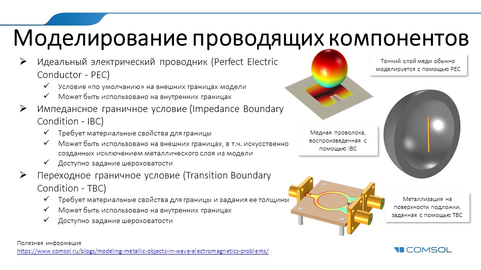
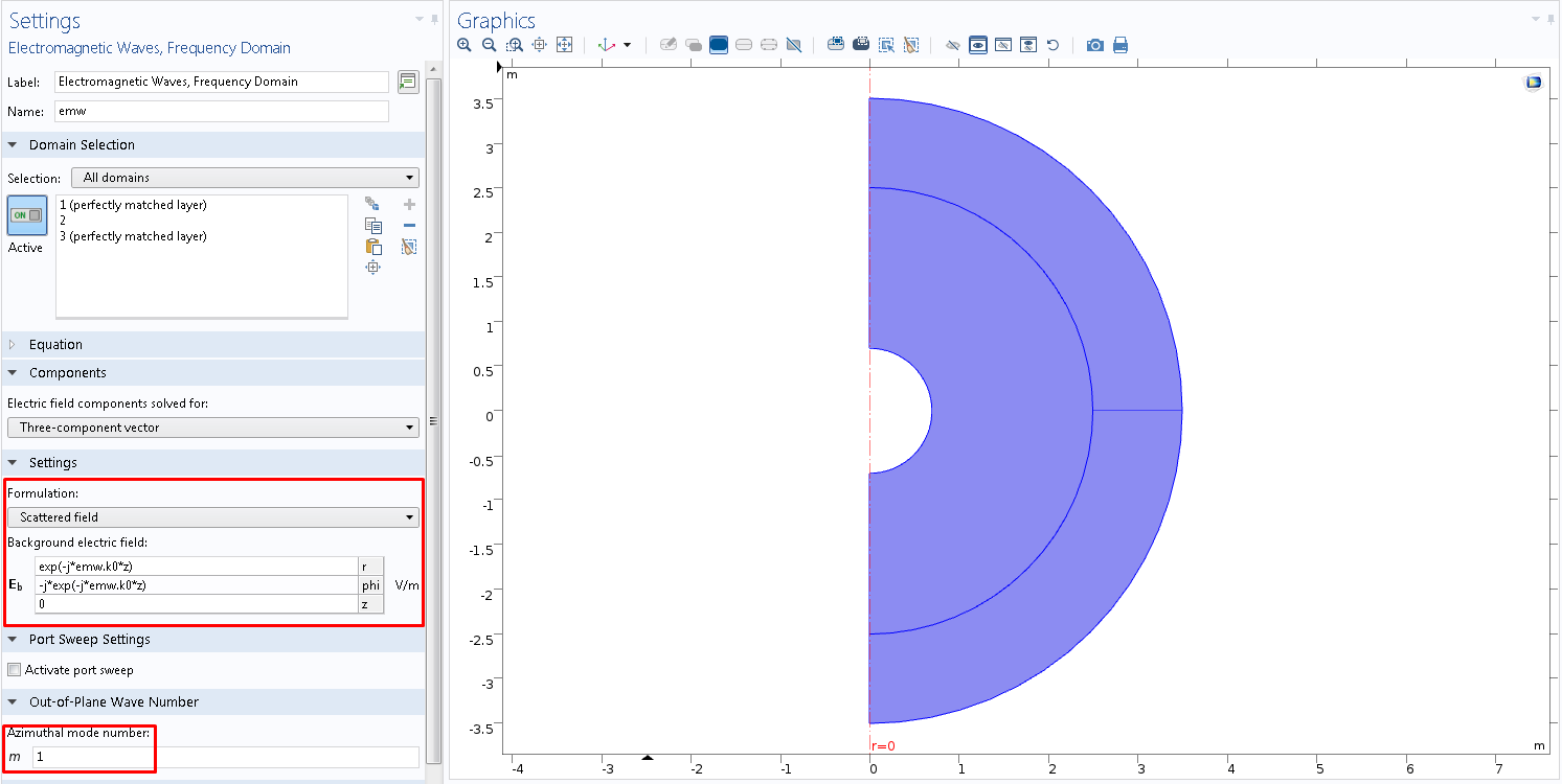
Fig. 3. Geometry for axisymmetric formulation and setting the background electromagnetic field with left circular polarization in the COMSOL Multiphysics ^® graphical interface .

In the computational domain (except for PML), the excitation of the background field with left circular polarization, directed in the negative direction of the z axis, is specified (Fig. 3). Please note that the calculation is made only for the first azimuth mode.

By default, for microwave tasks in COMSOL Multiphysics ^{®, a} free triangular (or tetrahedral for 3D problems) grid is automatically constructed for the frequency specified in the frequency domain (Frequency Domain study), which is 200 MHz in this example. To ensure sufficient resolution of wave processes in the model, the maximum size of the grid element is set equal to 0.2 wavelength. In other words, the spatial resolution is given as five second order elements per wavelength. In ideally matched layers, the grid is drawn by pulling in the direction of absorption, which ensures maximum efficiency of the PML.

Because the number of degrees of freedom in the model is very small (compared to the three-dimensional formulation), then its calculation takes only a few seconds. At the output, the user can receive and visualize the distribution of the electric field around the sphere (in the near zone), which is the sum of the background and diffuse fields.

For this task, the most interesting characteristics relate to the field of the far field. To get them in the model, you need to activate the Far-Field Calculation condition on the outer boundary of the computational domain (in this case, on the inner border of the PML), which allows you to calculate fields in the far zone outside the computational domain at any point based on the Stratton-Chu integral relations. The activation adds an additional variable — the field amplitude in the far field, on the basis of which engineering variables are computed in the post-processing software that meet IEEE standards: effective isotropically radiated power, gain (so-called Gain, including the input error) directional and EPR.

According to the polar graph, a specialist can determine the directionality of the field in the far zone in a certain plane, and a three-dimensional radiation pattern in the far zone allows us to study the stray field in more detail (Fig. 4).

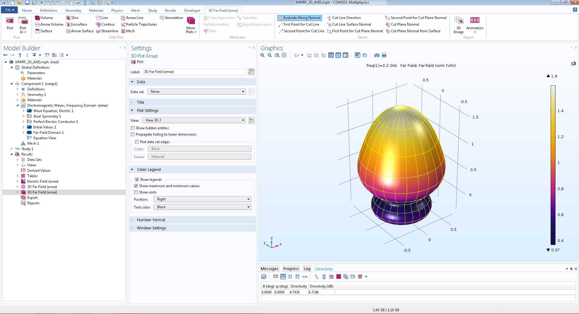
Fig. 4. Three-dimensional field visualization in the far field based on a two-dimensional axisymmetric model in COMSOL Multiphysics ^® .

Recovery solutions for three-dimensional problem

The results for the "reduced" model in axisymmetric formulation refer to the process of irradiating the conducting sphere with a background field with circular polarization. In the original 3d problem, the characteristics of the stray field are investigated for the case of a linearly polarized plane wave. How to circumvent this difference?

By definition, linear polarization can be obtained by adding the right and left circular polarization. A two-dimensional axisymmetric model with the above settings (Fig. 2) corresponds to the first azimuthal mode (m = 1) of the background field with left circular polarization. The solution for the negative azimuthal mode with the right circular polarization can be easily derived from the already solved problem, using the properties of symmetry and carrying out simple algebraic transformations.

Having carried out only one two-dimensional analysis and mirroring the results already in the process of post-processing, you can extract all the necessary data, saving significant computing resources (Fig. 5).

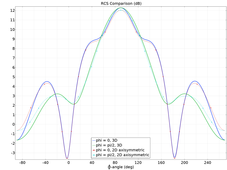
Fig. 5. Comparison of the sweep of the effective area of ​​dispersion (on a logarithmic scale) over the scattering angles for the full three-dimensional calculation and the proposed two-dimensional axisymmetric model.

A one-dimensional graph (Fig. 5) with a comparison of the EPR demonstrates acceptable correspondence between three-dimensional and two-dimensional axisymmetric models. A small discrepancy is observed only in the area of ​​forward and backscattering, near the axis of rotation.

In addition, visualization of the obtained two-dimensional results in three-dimensional space will require the transformation of a coordinate system from cylindrical to Cartesian . In fig. 6 shows a three-dimensional visualization of the results for a two-dimensional axisymmetric model.

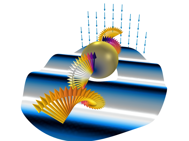
Fig. 6. Three-dimensional representation of the results obtained on the basis of a two-dimensional calculation.

Spiraling arrows indicate a circular polarized background field. The graph in the horizontal section is the distribution of the radial component of the background field (the wave process is mapped using plane deformations). On the surface of the sphere is built the norm of the full electric field. Another arrow diagram shows the superposition of two circular polarizations, which is equivalent to a background field with linear polarization in three-dimensional space.

Conclusion

In the process of modern development in the field of radiophysics and microwave engineering for engineers, effective modeling techniques that reduce resource consumption and time are irreplaceable, regardless of the numerical analysis method used.

To preserve the integrity and recreate all relevant physical effects when modeling a real component with a large electrical size, it is possible to simplify the process of numerical calculation without loss of accuracy by solving the problem in a two-dimensional axisymmetric formulation. When modeling and analyzing such axisymmetric objects as scattering spheres and disks, conical horn and parabolic antennas , calculations for the device section are performed several orders of magnitude faster than using the full three-dimensional model.

Basics of antenna modeling in COMSOL Multiphysics

Короткий видеообзор (на рус.), в котором демонстрируются примеры моделирования СВЧ-антенн с помощью модуля Радиочастоты, включая расчет частотных характеристик S-параметров и импеданса, диаграммы Смита, исследование согласования, расчет полей в дальней зоне, определение коэффициента направленного действия (Directivity) и коэффициента усиления (Gain). Кроме того, рассмотрены принципы использования симметрии, моделирования антенн в режиме приёма и комплексных расчетов систем разнесенных в пространстве приемников и передатчиков, оценки электромагнитных наводок на соседние антенны и многое другое.

At the same time, a simple two-dimensional statement allows you to quickly restore in three-dimensional space and investigate the scattering of the background field with linear polarization, as well as the radiation directivity in the far zone for antennas excited by the TE11 electric transverse mode of a circular waveguide.

Additional Information

This material is based on the article J.Munn. Fast Numerical Analysis of Scattering and Radar Cross Section , Microwaves & RF magazine, May 3, 2018

COMSOL Multiphsycics ^® functionality also allows you to simulate:

• Radar and radar objects of arbitrary shape
• Broadband scattering based on the DG-FEM technique (formulation in the time domain using explicit solvers and subsequent FFT transform)
• Scattering on 3D objects, in particular, on a nanoparticle placed on a dielectric substrate .

For a more detailed acquaintance with the possibilities of our package for the applications considered in this article, we invite you to participate in our new webinar "Solving scattering problems in COMSOL Multiphsycics ^® " , which will be held on August 22, 2018.

You can also request a demo version of COMSOL in the comments or on our website .

Final gif: