The increase in dynamic range when developing an optical reflectometer
Limited dynamic range is a property of almost any technique that we encounter in life. For example, when buying headphones, we come across this concept. You also have to take this parameter into account when working with photography, both with film and digital.
And in optical reflectometry there is the same concept. In this area, the dynamic range is equivalent to how long the OTDR can analyze. In the analysis of optics in PON networks, it also plays a large role, because Splitters with a high division coefficient produce a large attenuation and an appropriate dynamic range is required to “see” the cable behind the splitter.
I (not alone, of course, but in the group) had the opportunity to develop an optical reflectometer and I want to share my knowledge on this topic. Namely, an approach to increasing the dynamic range.
To begin with, an OTDR with a dynamic range of 35/37 dB (meaning for 1550 and 1310 nm, respectively) is now not uncommon. The OTDR displays the optical power calculated on the basis of the formula 5 * log10 (P / Po) on the screen. Accordingly, the receiving part of an OTDR (amplifier path) operate in a power range from about 1 mW to (attention!) 0.1 nW (10 ^ -10 W). Seven orders of magnitude, 10e6! By the way, OTDRs with a range of 42 dB are now being produced. How to achieve such characteristics?
We will not consider the issue of “pulling out" a signal from noise (nano-watts is a very small quantity, comparable with noise in the circuit), because This is a topic for a separate discussion. And we will assume that the laser in our reflectometer is quite powerful, because it is so.
Now let's digress from a specific area (not everyone has to develop analog amplifiers with a high dynamic range) and move on to more understandable and obvious things. Let's draw an analogy with photography.
There is a similar problem in photography. A huge range of brightness of the real world from light white to dark black can not be transmitted by any medium: neither film, nor a digital matrix. But I want to see a picture as close to reality as possible. Therefore, to achieve the desired result, an exposure fork is made - a series of frames is removed, each of which “covers” only part of the real dynamic range. The resulting images are combined into a final image and as a result we have an image with a high dynamic range.
There are a lot of articles on this topic, take, for example: see on Wikipedia . With pictures.
The described approach is also used in reflectometry. The optical cable to which the OTDR is connected during measurements does not quickly change its characteristics. This allows the OTDR to take many measurements, “study” the cable before the picture appears on the screen.
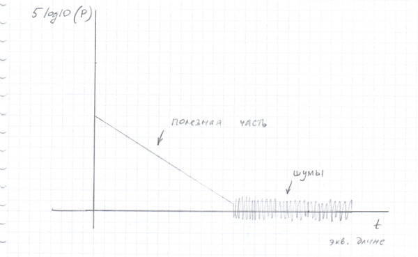
First, a series of measurements is done on the amplifier channel with a minimum gain. This amplifier "works out" a signal with high power. A weak signal does not fall into the range of this amplifier.
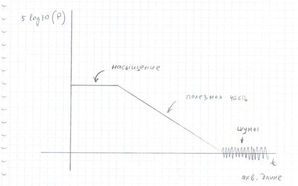
Then a series of measurements is made on the amplifier channel with a larger coefficient. This amplifier already "creeps" into the range of weaker signals, but loses information about a strong signal, since saturation occurs on a strong one. Notice the behavior is the same as the matrix / film in the photo.
Etc.
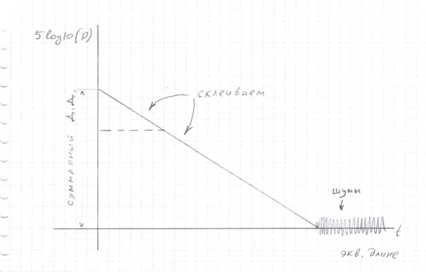
It turns out a set of measurements that need to be combined among themselves. Combining is not a big problem, although it is difficult to call this algorithm simple, given the variation in the characteristics of the circuit. Gain factors are well known and well known are those parts of the signal in which saturation has occurred.
And in optical reflectometry there is the same concept. In this area, the dynamic range is equivalent to how long the OTDR can analyze. In the analysis of optics in PON networks, it also plays a large role, because Splitters with a high division coefficient produce a large attenuation and an appropriate dynamic range is required to “see” the cable behind the splitter.
I (not alone, of course, but in the group) had the opportunity to develop an optical reflectometer and I want to share my knowledge on this topic. Namely, an approach to increasing the dynamic range.
To begin with, an OTDR with a dynamic range of 35/37 dB (meaning for 1550 and 1310 nm, respectively) is now not uncommon. The OTDR displays the optical power calculated on the basis of the formula 5 * log10 (P / Po) on the screen. Accordingly, the receiving part of an OTDR (amplifier path) operate in a power range from about 1 mW to (attention!) 0.1 nW (10 ^ -10 W). Seven orders of magnitude, 10e6! By the way, OTDRs with a range of 42 dB are now being produced. How to achieve such characteristics?
We will not consider the issue of “pulling out" a signal from noise (nano-watts is a very small quantity, comparable with noise in the circuit), because This is a topic for a separate discussion. And we will assume that the laser in our reflectometer is quite powerful, because it is so.
Now let's digress from a specific area (not everyone has to develop analog amplifiers with a high dynamic range) and move on to more understandable and obvious things. Let's draw an analogy with photography.
There is a similar problem in photography. A huge range of brightness of the real world from light white to dark black can not be transmitted by any medium: neither film, nor a digital matrix. But I want to see a picture as close to reality as possible. Therefore, to achieve the desired result, an exposure fork is made - a series of frames is removed, each of which “covers” only part of the real dynamic range. The resulting images are combined into a final image and as a result we have an image with a high dynamic range.
There are a lot of articles on this topic, take, for example: see on Wikipedia . With pictures.
The described approach is also used in reflectometry. The optical cable to which the OTDR is connected during measurements does not quickly change its characteristics. This allows the OTDR to take many measurements, “study” the cable before the picture appears on the screen.
First, a series of measurements is done on the amplifier channel with a minimum gain. This amplifier "works out" a signal with high power. A weak signal does not fall into the range of this amplifier.
Then a series of measurements is made on the amplifier channel with a larger coefficient. This amplifier already "creeps" into the range of weaker signals, but loses information about a strong signal, since saturation occurs on a strong one. Notice the behavior is the same as the matrix / film in the photo.
Etc.
It turns out a set of measurements that need to be combined among themselves. Combining is not a big problem, although it is difficult to call this algorithm simple, given the variation in the characteristics of the circuit. Gain factors are well known and well known are those parts of the signal in which saturation has occurred.