Where and how to get into embeddingings of graphs

Hi, Habr!

Three years ago on the site of Leonid Zhukov, I poked a link to the course of Jura Leskoveka cs224w Analysis of Networks and now we will go along with everyone in our cozy chat channel # class_cs224w. Immediately after the warm-up with an open course of machine learning , which will begin in a few days.

Question: What do they recite?
Answer: Modern mathematics. We show an example of improving the process of IT-recruiting.

Under the cat a reader is waiting for the story of how the project manager of discrete mathematics brought to the neural networks, why ERP implementers and product managers should read the Bioinformatics magazine, how the problem of recommending communications appeared, who needed graph embeddings, and where they came from. how to stop being afraid of questions about trees at interviews, and what it all may cost. Let's go!

Our plan is:

  1) What is cs224w
  2) Checkers or go
  3) How did I get to all this
  4) Why read Bioinformatics magazine
  5) What are graph embeddings and where did they come from
  6) Random tramp in the form of a matrix
  7) Return of a random tramp and link strength
  8) The path of the random tramp and the top in the vector
  9) Our days are a random tramp for everyone
10) How and where to store such data and where to get
11) What to fear
12) Memo to the replicator

What is cs224w

The Course of Jure Leskoveka Analysis of Networks stands out in the pleiad of educational products from the Faculty of Computational Sciences at Stanford University. The difference from the others is that the program covers a very wide range of issues. It is an interdisciplinary character that makes adventure a challenge. The prize is the universal language for describing complex systems - graph theory, which is proposed to be dealt with in ten weeks.

The course does not cost itself that way, but opens the Mining Massive Data Sets Graduate Certificate program , in which there is still a lot of tasty.

The second in the adventure is CS229 Machine Learning by Andrew Un, who does not need to advertise.

This is followed by CS246 Mining Massive Data Sets Jure Leskoveka, in which wishing is invited to challenge MapReduce and Spark.

Chris Manning completes the CS276 Information Retrieval and Web Search Banquet.

As a bonus, CS246H Mining Massive Data Sets: Hadoop Labs is offered specifically for those who were few. Again, visiting Jura.

In general, they promise that those who have gone through the program will acquire skills and knowledge sufficient to search for information on the Internet (without any Google and others like them).

Ride or checkered

Once upon a time, my supervisor and mentor, at that time - the service station in the Ukrainian Nestlé, explained to me, a young and ambitious person, who was trying to get an MBA to become even more famous, the truth that in the labor market people buy and sell experience and knowledge, and not diplomas and test results.

The above specialization can be completed online for a symbolic $ 18,900.

On average, an adventure takes 1-2 years, but no more than 3. To obtain a certificate, you must complete all courses with a grade of at least B (3.0).

There is another way.

All materials of the courses Jure Leskoveka are published openly and very quickly. Therefore, those who wish can suffer at any convenient time, coordinating the load with their abilities. Especially gifted I recommend to try the adventure mode "This is Stanford, honey!" - passing parallel to the course - videos of lectures spread in a couple of days, additional literature is available immediately, homework and solutions open gradually.

In this season, after the open course learning machine Habré , who is useful to go through as a warm-up, we'll have a race in a dedicated channel # class_cs224w chat ods.ai .

It is recommended to have the following skill set:

Basics of computational sciences at a level sufficient for writing non-trivial programs.
Fundamentals of probability theory.
Basics of linear algebra.

How I got to it all

He lived for himself, did not hurt. Led SAP implementation projects . At times, he acted as a playing coach in his main specialization, and he turned the CRM nuts. You can say almost did not touch anyone. Self-education involved. At some point I decided to specialize in the field of business transformation.(or making organizational changes). The task of analyzing organizations before and after change is an important part of this work. Knowing where and where to change - it helps a lot. Understanding the connections between people is a significant success factor. He spent several years studying the “soft” methodologies of research of organizations, but he couldn’t be satisfied with the question: “And who will fence whom: the chief accountant of the main account, or is everyone stronger?” I have been asking myself for several years in a row Everything is looking for a way to measure for sure.

The year 2014 was a turning point, when I gave up on MBA dreams and chose (here is the drum roll) again statistics and information management at the new University of Lisbon (the first and still healthy department of telecommunications of the non-existent Aviation and Space Systems Department of the Kiev Polytechnic) + Department of Communications at the military commissary).

In the first semester of the second magistracy, I tried out the analysis of social networks - one of the applications of graph theory. It was then that I found out that it’s what, it turns out, there are algorithms that solve problems like who will be friends with someone against the introduction of new technologies, but I didn’t know before and dried my head, analyzing people's connections in their mind - She really swells from this. Quite by chance, it turned out that the analysis of networks, after the first steps, is a complete data digging and machine learning, then with a teacher, now without.

At first, enough of the classics.

I wanted more. In order to deal with embeddings (and work Marinka Zhitnik for my tasks ), I had to delve into deep learning, in which the Deep Learning course helped me with my fingers . Considering the speed with which the Leskoveka group creates new knowledge, in order to solve administrative tasks automatically, it is enough just to follow their work.

Why read Bioinformatics magazine

Team building is not an easy task. Anyone with whom in one boat is not worth planting - one of the pressing issues. Especially when the faces are new. And the area is unfamiliar. And to lead to distant shores you need not one boat, but a whole flotilla. And on the way, close interaction is necessary both in the boats and between them. Everyday SAP implementation , when the Customer needs to put the system configured for its specificity from a heap of modules, and the project plan consists of thousands of lines. For all my work, I never hired anyone - they always gave out a team. You are the project manager, you have the authority, and you’re going around. Something like this. Twisted.

Example from the life:

I did not interview myself, but I selected the Timlides for this. And for the resources - the demand from me. And the integration of new team members is also the responsibility of the project manager. I think many will agree that the better the list of candidates is prepared, the more pleasant the process for all participants. This problem we consider in detail.

Natural laziness required - find a way to automate. Found. I share.

A bit of management theory. Adizes’s methodology is based on a basic principle: organizations, like living organisms, have their own life cycle and demonstrate predictable and repetitive behavioral manifestations in the process of growth and aging. At each stage of organizational development, the company expects a specific set of problems. How well the management of the company copes with them, how successfully it implements the changes necessary for a healthy transition from stage to stage, and determines the ultimate success or failure of this organization.

I have known about the ideas of Yitzhak Adizes for ten years and in many respects agree.

Personality of employees - like vitamins - affect success in certain conditions. There are examples of how successful executives, moving from one industry, failed to another. It could be worse. For example, Marissa Mayer, who raised Google search, dropped Yahoo. Warren Buffett says that he would hardly have been successful if he was born in Bangladesh. The environment and the ways of interaction in it are an important factor.

It would be good to predict complications before experiments on live, right?

This is the outline of another Marinka Zhitnik research published in the journal Bioinformatics. The task of predicting side effects with the joint use of drugs is mathematically close to the management. All thanks to the universality of the graph language. Consider it in more detail.

Decagon graph convolution network is a tool for predicting links in multimodal networks.

The method consists in the construction of a multimodal graph of protein-protein, drug-protein interactions, and side effects from a combination of drugs, which are represented by drug-drug connections, where each of the side effects is a certain type of rib. Decagon predicts a specific type of side effect, if any, which is manifested in the clinical picture.

The figure shows an example of a side effect graph derived from genome and population data. In total, there are 964 different types of side effects (indicated by ribs of type ri, i = 1, ..., 964). Additional information in the model is presented in the form of vectors of properties of proteins and drugs.

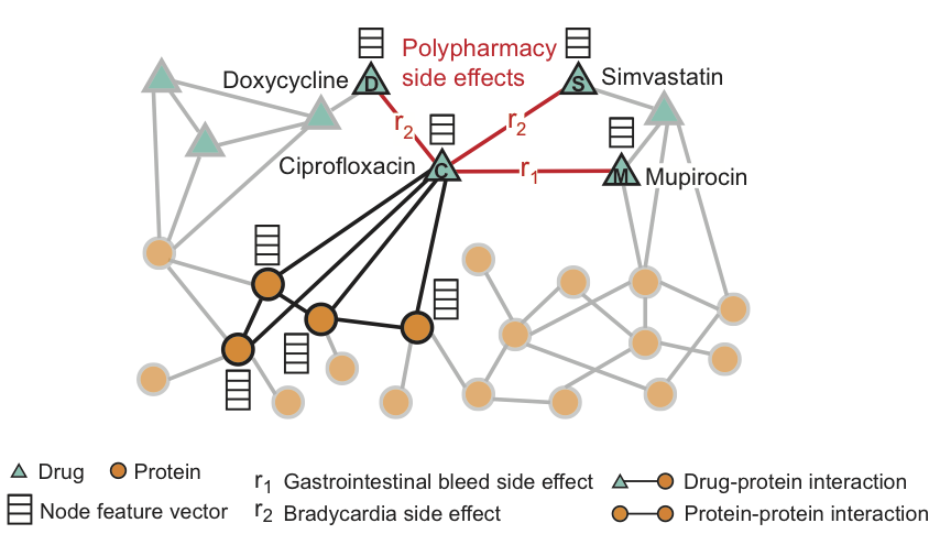
For Ciprofloxacin (node C), highlighted neighbors in the graph reflect the effects on four proteins and three other drugs. We see that Ciprofloxacin (node C), taken simultaneously with Doxycycline (node D) or Simvastatin (node S), increase the risk of a side effect expressed in slowing heart rate (side effect of r2 type), and the combination with Mupirocin (M) - increases the risk of gastrointestinal bleeding (side effect of type r1).

Decagon predicts associations between drug pairs and side effects (shown in red) to identify side effects from a simultaneous dose, i.e. those side effects that can not be associated with any of the drugs from the pair separately.

Decagon graph convolutional neural network architecture:

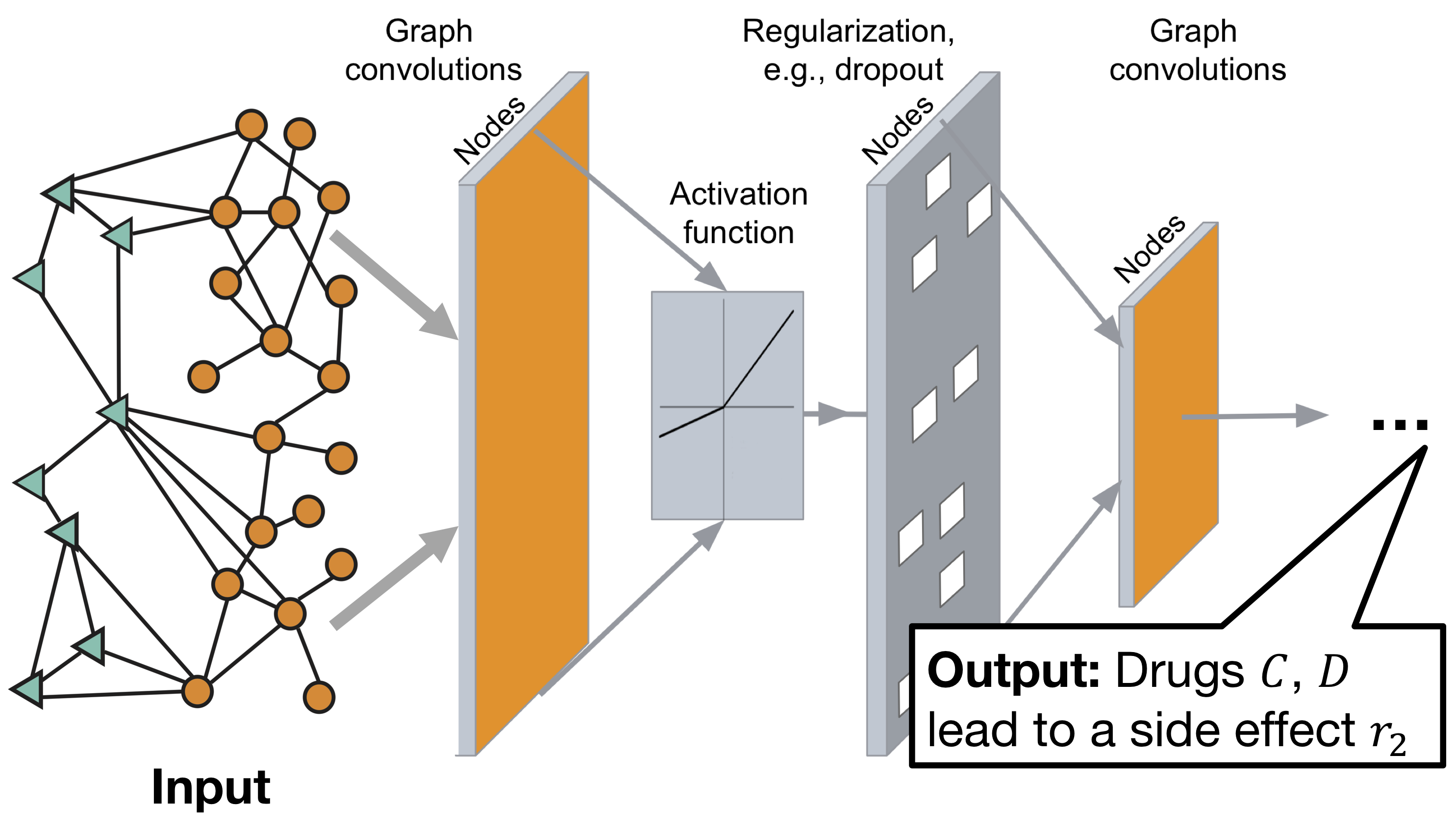
The model consists of two parts:

Encoder: graph convolutional network (GCN) receiving graph and producing embeddings for nodes;
Decoder: tensor factorization model using these embeddings to identify side effects.

More information can be found on the project website or below.

Great, but how to fasten it to team building?

Something like that .

It is in order to feel comfortable in the field of research, similar to that described, and it is worth digging the granite of science. However, it is possible to dig intensively - graph theory is actively developing. That's why it is the point of progress - there are very few who are comfortable.

To understand the details of the functioning of the Decagon, let's take a look at the history.

What is graph embeddingings and where did they come from

I happened to observe a change in the set of advanced methods for solving problems of predicting relationships on graphs over the past four years. It was fun. Almost like in a fairy tale - the further, the worse. Evolution went along the path from the heuristics, which determined the environment for the top of the graph, to random vagrants, then spectral methods appeared (matrix analysis), and now neural networks.

We formulate the problem of predicting relationships:

Consider an undirected graph $$ inline $ \ begin {align *} G (V, E) \ end {align *} $ inline $$ where
$$ inline $ \ begin {align *} V \ end {align *} $ inline $$ - many vertices $$ inline $ \ begin {align *} v \ end {align *} $ inline $$ ,
$$ inline $ \ begin {align *} E \ end {align *} $ inline $$ - many ribs $$ inline $ \ begin {align *} e (u, v) \ end {align *} $ inline $$ connecting vertices $$ inline $ \ begin {align *} u \ end {align *} $ inline $$ and $$ inline $ \ begin {align *} v \ end {align *} $ inline $$ .

Define the set of all possible edges. $$ inline $ E ^ {\ diamond} $ inline $$ its power
$$ inline $ \ begin {align *} | E ^ {\ diamond} | & = \ frac {| V | * (| V | - 1)} {2} \\ \ end {align *} $ inline $$ where
$$ inline $ \ begin {align *} | V | = n \ end {align *} $ inline $$ - the number of vertices.

Obviously, many non-existent edges can be expressed as $$ inline $ \ begin {align *} \ overline {E} = E ^ {\ diamond} - E \ end {align *} $ inline $$ .

We assume that in the set $$ inline $ \ begin {align *} \ overline {E} \ end {align *} $ inline $$ there are missing links, or links that will appear in the future, and we want to find them.

The solution is to define the function. $$ inline $ \ begin {align *} D (u, v) \ end {align *} $ inline $$ distance between the vertices of the graph, allowing for the structure of the graph $$ inline $ \ begin {align *} G (t_0, t_0 ^ \ star) \ end {align *} $ inline $$ given on the time interval $$ inline $ \ begin {align *} (t_0, t_0 ^ \ star) \ end {align *} $ inline $$ predict the appearance of ribs $$ inline $ \ begin {align *} G (t_1, t_1 ^ \ star) \ end {align *} $ inline $$ in the interval $$ inline $ \ begin {align *} (t_1, t_1 ^ \ star) \ end {align *} $ inline $$ .

One of the first publications that suggests moving from clustering to the problem of predicting relationships in the context of studying gene co-expression appeared in Bioinformatics in 2000 (as you might guess). Already in 2003, an article by John Kleinberg published an overview of current methods for solving the problem of predicting social network connections. His book " Networks, Crowds, and Markets: Reasoning About a Highly Connected World " is a textbook that is recommended to read during the cs224w course, most chapters are listed in the required reading section.

The article can be considered a slice of knowledge in a narrow field, as we see, at first the range of methods was small and included:

Methods based on neighbors in the graph - and the most obvious of them is the number of common neighbors.

We give the definition:

Vertex $$ inline $ u $ inline $$ is a neighbor in the graph for the top $$ inline $ v $ inline $$ if edge $$ inline $ e (u, v) \ in E $ inline $$ .

Denote $$ inline $ \ Gamma (u) $ inline $$ many vertex neighbors $$ inline $ u $ inline $$ ,

then the distance between the peaks $$ inline $ u $ inline $$ and $$ inline $ v $ inline $$ can be written as

$$ inline $ D_ {CN} (u, v) = \ Gamma (u) \ cap \ Gamma (v) $ inline $$ .

It is intuitively clear that the greater the intersection of the sets of neighbors of two peaks, the more likely the connection between them is, for example, most new acquaintances are with friends of friends.

More Advanced Heuristics - Jacquard Ratio $$ inline $ D_J (u, v) = \ frac {\ Gamma (u) \ cap \ Gamma (v)} {\ Gamma (u) \ cup \ Gamma (v)} $ inline $$ (who was already then one hundred years old) and recently (at that time) the proposed distance of Adamyk / Adar $$ inline $ D_ {AA} (u, v) = \ sum_ {x \ in \ Gamma (u) \ cap \ Gamma (v)} \ frac {1} {\ log | \ Gamma (x) |} $ inline $$ develop the idea through simple transformations.

Methods based on paths on a graph — the idea is that the shortest path between two vertices on a graph corresponds to the chance of a connection between them — the shorter the path, the higher the chance. You can go further and take into account not only the shortest, but all other possible paths between pairs of vertices, for example, weighing the paths, as the Katz distance does . Even then, the expected path length of the random tramp is mentioned - the forerunner of the basis of the method of recommending friends to Facebook.

Estimate the quality of the forecast:

For each pair of vertices $$ inline $ (u, v) $ inline $$ every non-existent edge $$ inline $ e (u, v) \ in \ overline {E} $ inline $$ calculate distance $$ inline $ D (u, v) $ inline $$ on the graph $$ inline $ G (t_0, t_0 ^ \ star) $ inline $$ .
Sort pairs $$ inline $ (u, v) $ inline $$ descending distance $$ inline $ D (u, v) $ inline $$ .
Will select $$ inline $ m $ inline $$ the pairs with the highest values are our prediction.
Let's see how many of the predicted edges appeared in $$ inline $ G (t_1, t_1 ^ \ star) $ inline $$ .

It is important to remember that the number of common neighbors and the Adamik / Adar distance are powerful methods that determine the basic level of forecast quality for the linkage structure alone, and if your recommendation system shows a weaker result, then something is wrong.

Generally, graph embeddings are a way of representing graphs compactly for machine learning tasks using the transform function $$ inline $ \ begin {align *} \ phi: G (V, E) \ longmapsto \ mathbb {R} ^ d \ end {align *} $ inline $$ .

We considered several of these functions, the most effective of the first. A broader list is described in the Kleinberg article. As we see from the review, even then they began to use high-level methods, such as matrix decomposition, pre-clustering, and tools from the arsenal of computational linguistics. Fifteen years ago, everything was just beginning. Embeds were one-dimensional.

Random tramp in the form of a matrix

The next milestone on the way to the graph embedding was the development of random walk methods. To invent and substantiate new formulas for calculating the distance, apparently, it became broke. In some applications, it seems, you just have to rely on chance and trust the hobo.

Let us give a definition: the

adjacency matrix of a graph $$ inline $ G $ inline $$ with finite number of vertices $$ inline $ n $ inline $$ (numbered from 1 to $$ inline $ n $ inline $$ ) - this is a square matrix $$ inline $ A $ inline $$ size $$ inline $ n \ times n $ inline $$ in which the value of the element $$ inline $ a_ {ij} $ inline $$ equal to weight $$ inline $ w_ {ij} $ inline $$ ribs $$ inline $ e (i, j) $ inline $$ .

Note: here we will deliberately move away from the previously used vertex indicators $$ inline $ u, v $ inline $$ and we will use the notation usual for linear algebra and in general in working with matrices $$ inline $ i, j $ inline $$ .

We illustrate the concepts considered:

Let $$ inline $ G $ inline $$ - four-vertex graph $$ inline $ \ {A, B, C, D \} $ inline $$ connected by ribs.

In order to simplify the construction, let us assume that the edges of our graph are bidirectional, i.e. $$ inline $ \ forall e (i, j) \ in E, \ exists e (j, i) \ in E \ land w_ {ij} = w_ {ji} $ inline $$ .

$$ inline $ e (A, B), w_ {AB} = 1; \\ e (B, C), w_ {BC} = 2; \\ e (A, C), w_ {AC} = 3; \ \ e (B, C), w_ {BC} = 1. $ inline $$

Draw the set of edges: $$ inline $ e $ inline $$ - blue, and $$ inline $ \ overline {E} $ inline $$ - green.

$$ inline $ \ begin {align *} A = \ left [\ begin {matrix} 0 & 1 & 3 & 0 \\ 1 & 0 & 2 & 1 \\ 3 & 2 & 0 & 0 \\ 0 & 1 & 0 & 0 \ end {matrix} \ right] \ end {align *} $ inline $$

Writing a graph in matrix form opens up interesting possibilities. To demonstrate them, let's take a look at the work of Sergey Brin and Larry Page, and look at how PageRank works - the algorithm for ranking graph vertices, which is still an important part of Google search.

PageRank - coined to search for the best pages on the Internet. A page is considered good if other good pages value it (refer to it). The more pages contain links to it, and the higher their ranking, the higher the PageRank for this page.

Consider the interpretation of the method using Markov chains .

We give the definition: The

degree of the vertex (degree) is the power of the set of neighbors:
$$ inline $ d_i = | \ Gamma (i) | $ inline $$ ,

There are in-degree and out-degree. For our example, they are equivalent.

We construct a weighted adjacency matrix, guided by the rule:
$$ inline $ \ begin {align *} M_ {ij} = \ left \ {\ begin {matrix} \ frac {1} {d_j} & \ forall i, j \ iff i \ in \ Gamma (j), \\ 0 & \ forall i, j \ iff i \ notin \ Gamma (j). \ end {matrix} \ right. \ end {align *} $ inline $$

$$ inline $ \ begin {align *} M = \ left [\ begin {matrix} 0 & \ frac {1} {3} & \ frac {1} {2} & 0 \\ \ frac {1} {2} & 0 & \ frac {1} {2} & 1 \\ \ frac {1} {2} & \ frac {1} {3} & 0 & 0 \\ 0 & \ frac {1} {3} & 0 & 0 \ end {matrix} \ right] \ end {align *} $ inline $$

Notice that the columns $$ inline $ M $ inline $$ must add up to 1 (i.e. $$ inline $ M $ inline $$ - "column stochastic matrix "). The elements of each column give the probability of moving from the top. $$ inline $ j $ inline $$ in one of the adjacent vertices on the graph $$ inline $ i \ in \ Gamma (j) $ inline $$ .

Let be $$ inline $ r_i $ inline $$ will be the PageRank value for the top $$ inline $ i $ inline $$ , in which $$ inline $ d_i $ inline $$ outgoing edges. Then we can express PageRank for her neighbor $$ inline $ j $ inline $$ as

$$$ display $$ r_j = \ sum_ {i \ to j} \ frac {r_i} {d_i} $$ display $$$

So each of the neighbors $$ inline $ i $ inline $$ tops $$ inline $ j $ inline $$ contributes to its PageRank, and its size is directly proportional to the authority of the neighbor (i.e. its PageRank), and inversely proportional to the size of the neighbor's environment.

We can and will keep the PageRank values for all vertices in the vector $$ inline $ \ begin {align *} r = [r_1, r_2, ..., r_n] ^ T \ end {align *} $ inline $$ - this will allow to write the equation compactly in the form of a scalar product:

$$$ display $$ r = Mr $$ display $$$

Imagine a web surfer who spends an infinite amount of time on the Internet (which is not far from reality). At any given time $$ inline $ t $ inline $$ it's on page $$ inline $ i $ inline $$ and at the moment $$ inline $ t + 1 $ inline $$ follows one of the links to one of the adjacent pages $$ inline $ j \ in \ Gamma (i) $ inline $$ , choosing it randomly, and all transitions are equally probable.

Denote $$ inline $ p (t) $ inline $$ vector with the probability that the surfer is on the page $$ inline $ i $ inline $$ at the moment of time $$ inline $ t $ inline $$ . $$ inline $ p (t) $ inline $$ - probability distribution between pages, therefore the sum of elements is equal to 1.

Recall that $$ inline $ M_ {ij} $ inline $$ - is the probability of transition from the top $$ inline $ j $ inline $$ to the top $$ inline $ i $ inline $$ given that the surfer is on top $$ inline $ j $ inline $$ and $$ inline $ p_j (t) $ inline $$ - the probability that it is on the page $$ inline $ j $ inline $$ in the moment $$ inline $ t $ inline $$ . Therefore, for each vertex $$ inline $ i $ inline $$

$$$ display $$ p_i (t + 1) = M_ {i1} p_1 (t) + M_ {i2} p_2 +. . . + M_ {in} p_n (t) $$ display $$$

and that means that

$$$ display $$ p (t + 1) = Mp (t) $$ display $$$

If random walks ever reach a state in which $$ inline $ p (t + 1) = p (t) $ inline $$ then $$ inline $ p (t) $ inline $$ - stationary distribution . Recall that the equation for PageRank in vector form $$ inline $ r = Mr $ inline $$ . Conclusion - Vector $$ inline $ r $ inline $$ PageRank values are the stationary distribution of the random tramp!

In practice for $$ inline $ r $ inline $$ PageRank equation is often solved by a power method . The idea is that we initialize the vector $$ inline $ r ^ {(t0)} = [1 / n, 1 / n, ..., 1 / n] ^ T $ inline $$ the same values and consistently calculate $$ inline $ r ^ {(t + 1)} = Mr ^ {(t)} $ inline $$ for each $$ inline $ t $ inline $$ until the values converge, i.e. $$ inline $ || r ^ {(t + 1)} - r ^ {(t)} || _1 <\ epsilon $ inline $$ where $$ inline $ \ epsilon $ inline $$ - allowable error. (Note that $$ inline $ || x || _1 = \ sum_ {k} | x_k | $ inline $$ - this $$ inline $ L_1 $ inline $$ norm, or Minkowski distance ). Then the values of the vector $$ inline $ r ^ {(t + 1)} $ inline $$ and will be an estimate of page rank for vertices. As a rule, 20-30 iterations are enough.

Here, the memoras about solving problems by random search acquires new shades.

In the “vanilla” form described, the method is sensitive to two problems:

T.N. "spider nests" - vertices that link to themselves - leads to the fact that PageRank flows into them. The whole. And no one else gets it.
Dead ends - vertices with only incoming edges - through them PageRank flows away from the system. And ends at some point. Vector $$ inline $ r $ inline $$ filled with zeros.

Bryn and Paige solved the problem 20 years ago by issuing a stroller~~shotgun~~ teleport!

Let our web surfer with probability $$ inline $ \ beta $ inline $$ selects the outgoing link, and with probability $$ inline $ 1 - \ beta $ inline $$ - Teleports to a randomly selected page. Usually meaning $$ inline $ 1 - \ beta \ approx 0.15 $ inline $$ i.e. our web surfer takes 5-7 steps between teleports. Out of the impasse - always teleport. The equation for PageRank takes the form:

$$$ display $$ r_j = \ sum_ {i \ to j} \ beta \ frac {r_i} {d_i} + (1- \ beta) \ frac {1} {n} $$ display $$$

(this formulation assumes that there are no dead ends in the column)

Like our previous matrix $$ inline $ M $ inline $$ we can define a new matrix

$$$ display $$ M ^ {\ star} = \ beta M + (1- \ beta) [1 / n] _ {n × n} $$ display $$$

transition probabilities. It remains to solve the equation $$ inline $ r = M ^ {\ star} r $ inline $$ in a similar way. For the sake of preserving intrigue, I’ll just say that the generalized algorithm is described on slides 37-38 in the 14th lecture of the 2017 cs224w course, in which Yura perfectly reveals all the details and shows how they use the method in Pinterest (it’s the main one in science) .

Let us return to the managerial affairs. What is the practical use of all these matrix operations?

Denote several tasks of the project manager:

Highlight key stakeholders ;
Identify the links between the project participants;
To pick up the participants of the groups that are most suitable for the teams.

The first task is solved by constructing a link graph and applying classical PageRank. For example, we caught Mr. Barack Obama from a correspondence that Mrs. Hillary Clinton kindly shared while other methods did not give him enough attention.

The remaining two will require modification of the algorithm.

The return of the random tramp and the power of connections

In the real world, it took eight years.

Recall that earlier our tramp with a teleport moved to a randomly selected vertex. But what if we limit the number of possible displacements to a non-random sample by some criterion? This was done in 2006 by fellow postgraduate colleagues Jura.

Let's improve our example: Suppose we know something about the vertices of the graph under consideration. $$ inline $ G $ inline $$ some signs.

For each vertex $$ inline $ i $ inline $$ set the vector from $$ inline $ k $ inline $$ properties $$ inline $ f ^ {(i)} = [f_1, f_2, ..., f_k] ^ T $ inline $$ .

Let the first of them $$ inline $ f_1 $ inline $$ there will be, say, a favorite eye color.

Suppose that the reader has reached the highest ranks and he already has a team that is working on the creation of a new revolutionary product. At some point there is a need to add one more player. Assume that the pool of candidates is quite extensive (for example, our uncle works in a datasaentist factory). In order to make life easier for our IT recruiter to create a list of those whom we invite to interview key team members (their time is also expensive) - we will solve it algorithmically.

Suppose the question we asked is to prepare a list of candidates ranked according to the criterion of potential compatibility, the most suitable for our two players, $$ inline $ A $ inline $$ and $$ inline $ C $ inline $$ - they are blue-eyed cute.

We know that previous successful cooperation is the key to the success of future cooperation.

Therefore, we will build a graph of dataseental relations from the history of team performances in competitions on any platform, like Kaggle or Hackerrank, which allows participants not only to measure mathematics, but also to communicate on forums, put huskies and all that ).

We give a definition:

Personalized sample $$ inline $ S_k (x) $ inline $$ by value $$ inline $ x $ inline $$ criteria $$ inline $ k $ inline $$ let's call a subset of graph vertices $$ inline $ G $ inline $$ :

$$ inline $ \ forall i \ in V, i \ in S_k (x) \ iff f ^ {(i)} _ {k} = x $ inline $$

It remains to build a personalized transition probability matrix:

$$ inline $ \ begin {align *} M ^ {p} _ {ij} = \ left \ {\ begin {matrix} \ beta M_ {ij} + \ frac {1- \ beta} {| S_k (x) | } & \ forall i, j \ iff i \ in S_k (x), \\ \ beta M_ {ij} & \ forall i, j \ iff i \ notin S_k (x). \ end {matrix} \ right. \ end {align *} $ inline $$

And solve the equation $$ inline $ \ begin {align *} r = M ^ {p} r \ end {align *} $ inline $$ regarding $$ inline $ \ begin {align *} r \ end {align *} $ inline $$ , as we have done more than once. In vector $$ inline $ \ begin {align *} r \ end {align *} $ inline $$ contains the values of personalized PageRank in relation to our sample - the most relevant vertices. To resolve the issue of finding potential candidates, sort the content $$ inline $ \ begin {align *} r \ end {align *} $ inline $$ descending values - we are interested in the top of the list.

This method is responsible for preparing 80% of the recommendations in Pinterest.

Special case when $$ inline $ \ begin {align *} | S_k (x) | = 1 \ end {align *} $ inline $$ , called Random Walks with Restarts - tramps come back and return to one of the top of interest. As a result, we get a measure of proximity for each vertex of the graph with respect to that unique one. And this solves the problem of predicting relationships better than the Adamik / Adar distance allows.

Add more improvements:

Recall that the edges $$ inline $ \ begin {align *} e (i, j) \ in E \ in G \ end {align *} $ inline $$ our graph have weight $$ inline $ \ begin {align *} w_ {ji} \ end {align *} $ inline $$ .

This will allow you to specify a weighted matrix. $$ inline $ \ begin {align *} M ^ w \ end {align *} $ inline $$ transition probabilities:

$$ inline $ \ begin {align *} M ^ {w} _ {ij} = \ left \ {\ begin {matrix} \ frac {w_ {ij}} {\ sum_ {j} w_ {ij}} & \ forall i, j \ iff e (i, j) \ in E, \\ 0 & \ forall i, j \ iff e (i, j) \ notin E. \ end {matrix} \ right. \ end {align *} $ inline $$

The tramp will make the transitions, as before, by chance, but no longer equally likely!

The attentive reader has already wondered how to measure these weights.

This also puzzled Facebook in 2011. It was necessary to build a system of recommending friends from friends of friends, so much so as to maximize the creation of new connections. And the first step was to create a weighted graph of connections between users from the information in their profiles and interaction history (likes, messages, shared photos, etc.). Somehow the power of friendship on the Internet to measure.

$$$ display $$ w_ {ij} = f ^ w (i, j) = e ^ {- \ sum_ {z} {\ xi_z x_ {ij} [z]}}, $$ display $$$

Where $$ inline $ \ begin {align *} x_ {ij} \ end {align *} $ inline $$ - vector of properties of vertices and edges connecting them, i.e. $$ inline $ \ begin {align *} x_ {ij} = f ^ {(i)} \ cup f ^ {(j)} \ cup f ^ {e (ij)} \ end {align *} $ inline $$ , but $$ inline $ \ begin {align *} \ xi \ end {align *} $ inline $$ - vector of weights to be learned from the data.

Here the prepared reader will recognize the linear model , and the unprepared one will think that it is worth going through an open machine learning course to deal with the gradient descent, with which we will learn the values of weights in the vector $$ inline $ x_ {ij} $ inline $$ - they will show how likes and messages affect online friendships.

Why do we need all this?

Besides the fact that this approach allows us to predict connections even better, we can learn the rules of successful team building. And find out what to look for in the future.

Recall the conditions of our exercise. We observe the development of cooperation (joint participation in competitions) in the group of conditional datasainists on the interval $$ inline $ \ begin {align *} (t_0, t_0 ^ \ star) \ end {align *} $ inline $$ (for example, one calendar month) and we want to predict team building in the interval $$ inline $ \ begin {align *} (t_1, t_1 ^ \ star) \ end {align *} $ inline $$ (another month). In addition to participating in competitions, we monitor communication on the forums, huskies of kernels, and something else that pleases. All collected information is stored in the matrix $$ inline $ X ^ {\ star} \ in \ mathbb {R} ^ {(2k + l) \ times | E |} $ inline $$ (its columns are vectors $$ inline $ x_ {ij} $ inline $$ , $$ inline $ k, l $ inline $$ - dimensions of vectors of properties of vertices and edges $$ inline $ f ^ {(i)}, f ^ {e (ij)} $ inline $$ , respectively) and column $$ inline $ \ begin {align *} G \ end {align *} $ inline $$ for two time intervals.

Prepare data for machine learning.

For each vertex $$ inline $ \ begin {align *} i \ end {align *} $ inline $$ :

1) we define many friends of friends:

$$$ display $$ \ Gamma ^ {fof} (i) = \ bigcup_ {j \ in \ Gamma (i)} \ Gamma (j) - \ Gamma (i) $$ display $$$

2) and build sub-graphs $$ inline $ \ begin {align *} G ^ {fof} (i) \ end {align *} $ inline $$ connections with friends and friends of friends, $$ inline $ \ begin {align *} \ forall e (x, y) \ in E, e (x, y) \ in G ^ {fof} (i) \ iff x, y \ in \ Gamma ^ {fof} (i) \ cup \ Gamma (i) \ end {align *} $ inline $$

3) select the set of vertices, $$ inline $ \ begin {align *} D_i: \ {d_1, ..., d_k \} \ end {align *} $ inline $$ With whom connections were formed - these are our positive examples for learning,

4) all unresolved links from the set $$ inline $ \ begin {align *} \ overline {D_i} = \ Gamma ^ {fof} (i) - D_i \ end {align *} $ inline $$ - These are our negative examples for learning.

image align = center

Our task is to choose such a vector of scales. $$ inline $ \ begin {align *} \ xi \ end {align *} $ inline $$ in which positive examples from many $$ inline $ \ begin {align *} D_i \ end {align *} $ inline $$ will get a higher Personalized PageRank value relative to $$ inline $ \ begin {align *} i \ end {align *} $ inline $$ than negative examples.

To do this, set the loss function, which will be minimized:

$$$ display $$ L = \ sum_ {i} \ sum_ {d \ in D_i, \ overline {d} \ in \ overline {D_i}} h (r _ {\ overline {d}} - r_ {d}) + \ lambda || \ xi || ^ 2, $$ display $$$

Where $$ inline $ h (x) = 0 \ iff x <0; h (x) = x ^ 2 \ iff x \ geqslant 0; $ inline $$ - penalty for violation of the conditions, $$ inline $ \ lambda $ inline $$ - strength $$ inline $ L_2 $ inline $$ regularization of scales $$ inline $ \ xi $ inline $$ , $$ inline $ r $ inline $$ - vector with solutions of the equation $$ inline $ r = M ^ wr $ inline $$ regarding $$ inline $ r $ inline $$ for the sub-graph of friends of friends of a single vertex $$ inline $ i $ inline $$ .

The fun part is that the gradient of this function is calculated in the same way as PageRank by a power method. Details - in the 17th lecture edition 2014, slides 9-27.

That was the point of progress at the time of my first acquaintance with the course cs224w.

The path of the random tramp and the top in the vector

And then came the triumph of laziness!

It is known that the theory of graphs was invented by Leonard Euler, when he was bored with solving an unsolvable problem about the bridges that now stand in Kaliningrad. Instead of trying to dry his head for nothing, he invented a mathematical apparatus that allows one to prove the fundamental impossibility of solving a puzzle.

In the best traditions of computational sciences, we will also be lazy and set ourselves the task of finding a function that would allow us to move away from one-dimensional representations of nodes and move on to multidimensional property vectors.

Here we get to know graph embeds in the modern sense of the term.

Formally, we want:

1) Determine the encoder (the ENC match function, which specifies the node transform $$ inline $ u $ inline $$ in vector $$ inline $ z_u $ inline $$ );
2) Determine the similarity function of the nodes (measure of proximity in the graph, which we will apply to the encoder input);
3) Optimize the parameters of the encoder in such a way that:

$$$ display $$ similarity (u, v) \ approx z_ {v} ^ {T} z_v $$ display $$$

We strive to ensure that vertices closely located in the graph receive a close representation in the vector map. In other words, so that the angle between the two vectors obtained is minimal.

Great, but how to define it, this proximity in the graph?

For example, we will assume that the edge weight is a good measure of proximity and can be approximately considered equal to the scalar product for embeddings of two nodes. The loss function for such a case takes the form:

$$$ display $$ L = \ sum _ {(u, v) \ in V \ times V} || z_ {u} ^ {T} z_v - A_ {u, v} || ^ 2, $$ display $$$

it remains to find (for example, a gradient descent) matrix $$ inline $ Z \ in \ mathbb {R} ^ {d \ times | V |} $ inline $$ which minimizes $$ inline $ L $ inline $$ .

An alternative approach is to define the environment. $$ inline $ N (v) $ inline $$ for vertex wider than many neighbors.

This will help us wander on the graph. The first project to use this approach is DeepWalk . The essence of the method lies in the fact that we will run a vagabond walking on the graph randomly from each vertex $$ inline $ v $ inline $$ , and feed short sequences of fixed length visited tops during word walk in word2vec.

Here, the intuition is that the probability distribution of visits to the vertices of the graph — a power law — is very similar to the probability distribution of the appearance of words in human languages. And since word2vec works for words, it can also for graphs. Tried it - it worked out!

In DeepWalk, a tramp implements a first-order Markov process — we move from each vertex to the neighboring ones, according to probabilities from a weighted adjacency matrix $$ inline $ M $ inline $$ (or its derivatives, like $$ inline $ M ^ w $ inline $$ ). Where we came to the top does not affect the choice of the next step.

In order to realize walks, you need a pseudo-random number generator and a little algebra . It's time to use the block for quotations for its intended purpose.

“Anyone who agrees with the arithmetic methods of generation is, of course, sinful. As has been repeatedly shown, there is no such thing as a random number — there are only methods for creating such numbers, and a rigid arithmetic procedure, of course, is not such a method ... We are only dealing with cooking recipes for creating numbers ... ”

- John von Neumann

It remains to advise those seeking to live a righteous life to find the album “Black and White Noise” on sale - in 1995 George Marsaglia recorded an array of bytes on a CD, obtained by digitizing the noise from the amplifier while playing the repchik and named it accordingly.

The development of the method is node2vec , which implements a second-order Markov process - we look where we came from, and this affects the probabilities of choosing the direction of the next step. Consider how this works.

Let's say we run a stroller to walk along the graph from the top $$ inline $ u $ inline $$ adjacent to its top $$ inline $ s_1 $ inline $$ tops $$ inline $ s_2 $ inline $$ and $$ inline $ w $ inline $$ - in two steps, and $$ inline $ s_3 $ inline $$ - in three. After each step, we can perform one of three possible actions: 1) return closer to $$ inline $ u $ inline $$ ; 2) explore vertices at the same distance from $$ inline $ u $ inline $$ as the one in which we are now; 3) move away from $$ inline $ u $ inline $$ .

This strategy is implemented using two parameters:
$$ inline $ p $ inline $$ - sets the probability to return to the previous vertex;
$$ inline $ q $ inline $$ - sets the balance between search in breadth and search deep.

These parameters define unregulated transition probabilities as follows:

Let's say we are at the top $$ inline $ w $ inline $$ and came into it from the top $$ inline $ s_1 $ inline $$ . For rib $$ inline $ e (w, s_1) $ inline $$ we will assign a weight (unrated probability) $$ inline $ 1 / p $ inline $$ . For rib $$ inline $ e (w, s_2) $ inline $$ - $$ inline $ 1 $ inline $$ (as for all other edges leading to the vertices equidistant from $$ inline $ u $ inline $$ ). For leading away from $$ inline $ u $ inline $$ ribs $$ inline $ e (w, s_3) $ inline $$ - $$ inline $ 1 / q $ inline $$ .

Then, we normalize the probabilities (so that the sum is equal to 1) and complete the next step.

We are interested in the sequence of visited vertices - we will send it to word2vec ( this article will help you to deal with it , or lecture 8 of the Deep Learning course on your fingers ). Selection of strategies for the vagabond, optimal for solving specific problems - the area of active research. For example, node2vec, with which we have become familiar, is a champion in the classification of vertices (for example, determining the toxicity of drugs, or gender / age / race of a social network member).

We will optimize the probability of the appearance of vertices on the tramp's path, the loss function:

$$$ display $$ L = \ sum_ {u \ in V} \ sum_ {v \ in N_ {R} (u)} -log (P (v | z_u)) $$ display $$$

in its explicit form, a rather expensive computational pleasure

$$$ display $$ L = \ sum_ {u \ in V} \ sum_ {v \ in N_ {R} (u)} -log (\ frac {e ^ {z_ {u} ^ {T} z_v}} { \ sum_ {n \ in V} e ^ {z_ {u} ^ {T} z_n}}), $$ display $$$

which, by happy coincidence, is solved by negative sampling , since

$$$ display $$ log (\ frac {e ^ {z_ {u} ^ {T} z_v}} {\ sum_ {n \ in V} e ^ {z_ {u} ^ {T} z_n}}) \ approx log (\ sigma (z_ {u} ^ {T} z_v)) - \ sum_ {i = 1} ^ {k} log (\ sigma (z_ {u} ^ {T} z_ {n_i})), \\ where \, \, \, n_i \ sim P_V, \ sigma (x) = \ frac {1} {1 + e ^ {- x}}. $$ display $$$

So, we figured out how to get a vector representation of the vertices. In the bag!

How to prepare edge embeddings:

We need to define an operator that allows for any pair of vertices. $$ inline $ u $ inline $$ and $$ inline $ v $ inline $$ build vector representation $$ inline $ z _ {(u, v)} = g (z_u, z_v) $ inline $$ regardless of whether they are related on the graph. Such an operator can be:

a) arithmetic average: $$ inline $ [z_u \ oplus z_v] _i = \ frac {z_u (i) + z_v (i)} {2} $ inline $$ ;
b) the work of Hadamard: $$ inline $ [z_u \ odot z_v] _i = z_u (i) * z_v (i) $ inline $$ ;
c) weighted L1 norm: $$ inline $ || z_u - z_v || _ {\ overline {1} i} = | z_u (i) - z_v (i) | $ inline $$ ;
d) weighted L2 norm: $$ inline $ || z_u - z_v || _ {\ overline {2} i} = | z_u (i) - z_v (i) | ^ 2 $ inline $$ .

In experiments, the work of Hadamard behaves most steadily.

Just in case, remember the Free Lunch Theorem:

No algorithm is universal - it is worth checking out a few methods.

The development of node2vec is the OhmNet project , which allows you to merge several graphs into a hierarchy and construct embeddingings of vertices for different levels of hierarchy. It was originally designed to simulate the connections between proteins in different organs (and they behave differently depending on location).

An astute reader here will see similarities with organizational structure and business processes.

And we - let us return for example from the field of IT-recruiting - selection of candidates, the most suitable for the already established team. Earlier we considered unimodal connection graphs of conditional datasaentists, obtained from the history of interaction (in a unimodal graph, vertices and relations are of the same type). In reality, the number of social circles in which an individual can be included is more than one.

Suppose, in addition to the history of joint participation in competitions, we also collected information about how datasaientists communicated in our cozy chat room . Now we have two connection graphs, and OhmNet is great for solving the problem of creating embeddings from several structures.

Now - about the shortcomings of the methods built on shallow encoders - there is only one hidden layer inside word2vec, the weights of which are encoded. At the output, we get a vertex-vector correspondence table. All of these approaches have the following limitations:

Each vertex is encoded with a unique vector and the model does not imply the sharing of parameters;
We can encode only those vertices that the model saw during training — we cannot do anything for new vertices (except to re-train the encoder again);
The vectors of vertex properties are not taken into account.

From the indicated deficiencies are free graph convolution networks. We got to Decagon!

Our days are a random tramp for everyone

I was lucky to write the first trainee diploma about the tramp and protect it back in 2003, but I had to go through the classic way with deep learning to figure out what was under the hood. And it's funny there.

First, let's look at why standard deep learning methods are not suitable for graphs.

Counts are not seals for you!

The modern set of deep learning tools (multilayer, convolutional, and recurrent networks) is optimized for solving problems on fairly simple data — sequences and lattices. Graph - the structure is more complicated. One of the problems that will prevent us from taking the adjacency matrix and sending it to the neural network is isomorphism .

In our toy graph $$ inline $ G $ inline $$ consisting of vertices $$ inline $ \ {A, B, C, D \} $ inline $$ for constructing the adjacency matrix $$ inline $ A $ inline $$ , we assumed through numbering $$ inline $ \ {1,2,3,4 \} $ inline $$ . It is easy to see that we can number vertices differently, for example $$ inline $ \ {1,3,2,4 \} $ inline $$ , or $$ inline $ \ {4,1,3,2 \} $ inline $$ - each time receiving a new adjacency matrix of the same graph.

$$ inline $ \ begin {align *} A = \ left [\ begin {matrix} 0 & 1 & 3 & 0 \\ 1 & 0 & 2 & 1 \\ 3 & 2 & 0 & 0 \\ 0 & 1 & 0 & 0 \ end {matrix} \ right], \, A ^ {\ {1,3,2,4 \}} = \ left [\ begin {matrix} 0 & 3 & 1 & 0 \\ 3 & 0 & 2 & 0 \\ 1 & 2 & 0 & 1 \\ 0 & 0 & 1 & 0 \ end {matrix} \ right], \, A ^ {\ {4,1,3,2 \}} = \ left [\ begin {matrix} 0 & 1 & 2 & 1 \\ 1 & 0 & 0 & 0 \\ 2 & 0 & 0 & 3 \\ 1 & 0 & 3 & 0 \ end {matrix} \ right]. \ end {align *} $ inline $$

In the case of cats, our network would have to learn to recognize them with all possible permutations of rows and columns - that is also a problem. As an exercise, try to change the numbering of the points in the picture below so that when they are connected in series, the cat will turn out.

The next bad luck with graphs with ordinary neural networks is the standard input dimension. When we work with images, we always normalize the size of the image in order to feed it to the input of the network - it is of a fixed size. With graphs, such a focus will not work - the number of vertices can be arbitrary - to squeeze the connectivity matrix to a given dimension without losing information - that is another challenge.

The solution is to build new architectures, inspired by the structure of the graphs.

To do this, we use a simple two-step strategy:

For each vertex, we construct a computational graph using a tramp;
Collect and transform information about neighbors.

Recall that the properties of the vertices we store in vectors $$ inline $ f ^ {(u)} $ inline $$ - matrix columns $$ inline $ X \ in \ mathbb {R} ^ {k \ times | V |} $ inline $$ and our task is for each vertex $$ inline $ u $ inline $$ collect properties of adjacent vertices $$ inline $ f ^ {(v \ in N (u))} $ inline $$ to get embedding vectors $$ inline $ z_ {u} $ inline $$ . The computational graph can be of arbitrary depth. Consider the option with two layers.

The zero layer is the properties of the vertices, the first is the intermediate aggregation using a certain function (indicated by a question mark), the second is the final aggregation, which produces the embeddingings vectors of interest.

And what's in the boxes?

In the simple case - a layer of neurons and nonlinearity:

$$$ display $$ h ^ 0_v = x_v (= f ^ {(v)}); \\ h ^ k_v = \ sigma (W_k \ sum_ {u \ in N (v)} \ frac {h ^ {k-1} _v} {| N (v) |} + B_k h ^ {k-1} _v), \ forall k \ in \ {1, ..., K \}; \\ z_v = h ^ K_v, $$ display $$$

Where $$ inline $ w_k $ inline $$ and $$ inline $ b_k $ inline $$ - model weights, which we will learn by gradient descent, using one of the considered loss functions, and $$ inline $ \ sigma $ inline $$ - non-linearity, for example RELU: $$ inline $ \ sigma (x) = max (0, x) $ inline $$ .

And here we find ourselves at a crossroads - depending on the task at hand, we can:

study without a teacher and take advantage of any of the previously considered loss functions - vagrants, or ribs weight. The weights obtained will be optimized so that the vectors of similar vertices are placed compactly;
start training with a teacher, for example - solve the problem of classification, wondering if the drug will be toxic.

For the problem of binary classification, the loss function takes the form:

$$$ display $$ L = \ sum_ {v \ in V} y_v log (\ sigma (z_v ^ T \ theta)) + (1-y_v) log (1- \ sigma (z_v ^ T \ theta)), $ $ display $$$

Where $$ inline $ y_v $ inline $$ - vertex class $$ inline $ v $ inline $$ , $$ inline $ \ theta $ inline $$ - vector of scales, and $$ inline $ \ sigma $ inline $$ - non-linearity, for example sigmoid: $$ inline $ \ sigma (x) = \ frac {1} {1 + e ^ {- x}} $ inline $$ .

A trained reader here learns cross-entropy and logistic regression, and an unprepared one will think that it is worth going through an open machine learning course to feel comfortable with the task of classification , simple , and more advanced algorithms for solving it (including gradient boosting ).

And we will move on and consider the principle of operation of GraphSAGE - the forerunner of Decagon.

For each vertex $$ inline $ v $ inline $$ we will aggregate information from neighbors $$ inline $ u \ in N (v) $ inline $$ and her.

$$$ display $$ h ^ k_v = \ sigma ([W_k \ cdot AGG (\ {h ^ {k-1} _u, \ forall u \ in N (v) \}), B_k h ^ {k-1} _v]), $$ display $$$

Where $$ inline $ AGG $ inline $$ - generalized designation of the aggregation function - the main thing - differentiable.

Averaging: take the weighted average of the neighbors

$$$ display $$ AGG = \ sum_ {u \ in N (v)} \ frac {h ^ {k-1} _u} {| N (v) |}. $$ display $$$

Pulling: elementwise average / maximum value

$$$ display $$ AGG = \ gamma (\ {Qh ^ {k-1} _u, \ forall u \ in N (v) \}). $$ display $$$

LSTM: shake up the environment (do not mix!) And run in LSTM

$$$ display $$ AGG = LSTM ([h ^ {k-1} _u, \ forall u \ in \ pi (N (v))]). $$ display $$$

On Pinterest, for example, they stuffed multilayer perceptrons into it and rolled it into PinSAGE prod .

In solving the problem of predicting the functions of proteins in organs, the aggregator pooling and LSTM (which are forever) were especially notable. Consider it in more detail and give an analogy with the processes of team building and IT-recruiting.

Let's draw obvious parallels:

Introductory: organ and protein, the goal - to determine the function performed by this protein in this organ.
In the world of team building, introductory: project / division and specialist, the goal is to define a role in a team.

With the development of technology and the growing amount of data on interactions between substances, marking them with the help of people is a task beyond what can be done. It seems that technological singularity has already begun in certain areas of knowledge. For example, during one of my first presales, when we were selling a system for constructing shift schedules for several thousand support center employees, an assessment of complexity sunk into my head. One manager can equalize the load taking into account the types of hiring (permanent / temporary) employees, years of service, necessary skills, and other things - manually - for no more than 30 people.

In similar organs, proteins perform biologically similar functions.

The task is to determine the likelihood of performing one of the many functions (multi-label node
classification task) —one protein can perform several roles in different organs. Solution - use graphs of interactions between proteins in different organs. The properties of the peaks (proteins) will be their genetic structures and immunological signatures (these data are rather fragmentary and inaccessible for 42% of proteins). We train the GraphSAGE graph convolutional network, and we learn the weights common to all vertices - now we know the generalized rules for the aggregation of information about neighbors.

The resulting weights allow you to generate embeddings for previously unseen graphs!

And this allows us to determine the function of proteins in previously unexplored organs, which is a breakthrough for medicine, since not all studies can be carried out, leaving the object alive. This kind of information helps to develop new drugs of directional action, which is certainly great.

Now we have dealt with the details necessary to understand the functioning of the Decagon. Recall, the method consists in constructing a multimodal graph protein-protein interactions, protein-drug, or side effects of a combination of drugs that appear to drug-drug bonds, wherein each of the side effects - rib certain type ri . Each of the side effects is modeled in isolation. For each drug vertex, we build 964 (by the number of side effects) computational graphs.

Then, for each drug, a computational graph is constructed nonlinearly, combining the graphs obtained in the previous step with the drug-protein and protein-protein interaction graphs.

Formally, for each layer we compute

$$$ display $$ h ^ k_v = \ sigma (\ sum_rW ^ {k-1} _r (\ sum_ {u \ in N_r (v)} \ frac {h ^ {k-1} _u} {\ sqrt {| N_r (v) || N_r (u) |}} + \ frac {h ^ {k-1} _v} {| N_r (v) |})), $$ display $$$

Where $$ inline $ \ sigma $ inline $$ - non-linearity, for example RELU. As we see, Decagon used the simplest version of the graph convolutional network - a weighted sum. Obviously, nothing prevents us from complicating the model, just like GraphSAGE. The embeddingings of the vertices obtained on the final layer are fed to the input of the decoder, which returns the probabilities of the occurrence of each of the side effects when drugs are taken together.

Let's understand how this decoder functions.

His task is to reconstruct the marked edges in the graph, relying on learned embeddingings. Each type of edge is processed in its own way. For each three parameters $$ inline $ (u, r, v) $ inline $$ The decoder calculates the function:

$$ inline $ \ begin {align *} g (u, r, v) = \ left \ {\ begin {matrix} z ^ T_uD_ {r_i} RD_ {r_i} z_j & u, v - preparations; \\ z ^ T_uM_rz_v & u, v - drug \, and \, protein, \, or \, both \, proteins. \ end {matrix} \ right. \ end {align *} $ inline $$

and submits the result to a sigmoid to determine the probability of occurrence of an edge of a given type:

$$$ display $$ p ^ {uv} _ {r} = p ((u, r, v) \ in E) = \ sigma (g (u, r, v)), \ sigma (x) = \ frac {1} {1 + e ^ {- x}}. $$ display $$$

So, we have end-to-end encoder-decoder model, in which there are four types of parameters: (i) $$ inline $ W_r $ inline $$ - weights of neural networks for the aggregation of each type of relationship in the graph, (ii) $$ inline $ M_r $ inline $$ - matrix of parameters of drug-protein and protein-protein relations, (iii) $$ inline $ r $ inline $$ - the general matrix of parameters of side effects, and (iv) $$ inline $ D_ {r_i} $ inline $$ - matrix parameters of each side effect.

All these parameters are learned by gradient descent using the cross-entropy loss function and negative sampling to select non-existent edges.

Here you can breathe out - the next update of the progress point is expected in six months.

Summing up all the above, in complex systems with a bunch of interrelations that we model using graphs, the characteristic features are clearly manifested: 1) homophilia - like - attracts; and 2) the old rule “Tell me who your friend is and I will tell you who you are” is still relevant. It's great that in order to curb all this riot of connections, now you no longer need to burn nerve cells, but you can just take and count.

How and where to store such data and where to get it.

Briefly - in RAM - so faster.

My personal position regarding the processing of graphs in RAM on one machine is related to the fact that the size of structured data (namely, we build graphs from them) grows more slowly than the amount of available RAM for reasonable money. For example, all genome research conducted by humankind from the GenBank database will fit in 1 TB, and a car with such a memory size now costs about the same as a golf class car - a working tool for a sales representative driving through pharmacies. Cluster computation is great, but distributed triad counting for a large graph due to the need to coordinate and collect computation results takes several times (if not an order of magnitude) more time than the same operation in SNAP with commensurate computing power.

Consider a few tools available today and ways to work.

A sufficiently detailed description of possible constructions of points and lines in the eponymous work gives those involved in the creation of the first graph database Neo4j , in which the model of a graph with properties (property graph) is implemented.

This approach allows you to build a multimodal graph in which many different entities can be linked by different types of links. The working task that the teacher addressed immediately was to link together (i) business processes, (ii) relations between employees, and (iii) a project plan in which pieces of work — separate tasks — somehow affect the first two. It was possible to search for the answer independently.

An alternative example of such data is the article itself and all those involved in it:

In addition, the contribution of Neo4j to the industry is to create a declarative Cypher language that implements a graph model with properties and operates in a form similar to SQL, with the following data types: vertices, relationships, dictionaries, lists, integers, floating point, and binary numbers, and lines. An example of a query returning a list of films with Nicole Kidman:

MATCH (nicole:Actor {name:'Nicole Kidman'})-[:ACTED_IN]->(movie:Movie)
WHERE movie.year < $yearParameter
RETURN movie

Neo4j with crutches can be made to work in memory.

It is also worth mentioning Gephi - a convenient means of visualization and layout of graphs on the plane - the first network analysis tool from personally tested. With a stretch we can assume that in Gephi it is possible to implement a graph with the properties of vertices and edges, though it will not be very convenient to work with it, and the set of algorithms for analysis is limited. This does not detract from the merits of the package - for me it is in the first place in a series of visualization tools. Having mastered the internal format of GEXF data storage , you can create impressive images. Attracts the possibility of easy export to the web, as well as the opportunity to set properties for vertices and edges in time and get intricate animations as a result- so built routes of movement of salesmen from the sales data. All thanks to the layout of graphs on the map according to the coordinates of the vertices - the standard part of the package.

Now I spend most of my research analytically, drawing pictures at the finish.

My search for tools and data processing methods in complexly coupled systems continues. Three years ago I found a solution for working with multimodal graphs. The SNAP Jura Leskoveka Library is a tool that he developed for himself and has already measured a lot of things for him. I use Snap.py - the version for Python (a proxy for SNAP functions implemented in C ++) and a set of about three hundred available operations is enough for me in most cases.

Recently Marinka Zhitnik released MAMBO - a set of tools (inside - SNAP) for working with multimodal networks and a tutorial in the form of a series of Jupyter notebooks with an exemplary analysis of genetic mutations.

Finally, there is SAP HANA Graph - everything inside ML, SQL, OpenCypher is everything your heart desires.

In favor of SAP HANA, the fact that digging is likely to result in well-structured transaction data from ERP, and clean data is worth a lot. Another plus is the powerful tools for searching sub-graphs using predetermined patterns — a useful and difficult task, which I have not seen in other packages and used specialized programs . A free license for a developer provides a base of 1 GB in size - just enough to play around with fairly large networks. Funny challenge - a set of analytical algorithms out of the box - small, PageRank will need to be implemented independently. To do this, you need to master GraphScript - a new programming language, but these are trifles. As my slalom trainer said, for the master it is dust!

Now about where to get the data in order to build graphs out of them. Some ideas:

Public university repositories: Stanford - General and Biomedical , Colorado ;
Combine the project plan with the organizational structure and risk register;
Identify the links between product structure, technology, and user requirements;
Conduct a sociographic study in a team;
Come up with something of their own , inspired by last year's course projects cs224w.

What to fear

You could say there will be a final warning about the risks associated with this party.

As you understand, ladies and gentlemen, the task of the program is to reflect the state of affairs at the cutting edge of progress in a very productive and generously funded research group. It's like Leningrad , only about modern mathematics. Possible side effects:

Dunning-Kruger , modified, without a novice euphoria and a plateau of excellence. Leskoveka try catch up.
Boredom in the province by the sea. Of the 400 people in the course given by the apparat, they were forced to write a project, and to pass the exam in the first session during my second magistracy, one and a half counters went. The teachers in their research activities remained at the level of modularity and centrality measures. On mitapakh about the python and the data is also sad. In general, if you do not know how to entertain yourself, I warned.
Pride in Slavic accent in English.

Memo to the replicator

Hi, replicator!

In the adventure that Jura Leskovek gave us, you will need free time. The course consists of 20 lectures, four houses, each of which is recommended to allocate about 20 hours of recommended literature, as well as - an extensive list of additional materials that will allow you to make a first impression of the state of affairs on the cutting edge of progress in any of the topics covered.

To perform tasks, it is strongly recommended to use the SNAP library (in a sense, the entire course can be viewed as an overview of its capabilities).

In addition, you can try to implement your own project or write a tutorial on the topic you like.

Lecture summary for 2017:

1. Вступление и структура графов
Анализ сетей — это универсальный язык описания сложных систем и сейчас — самое время с ним разобраться. Курс акцентируется на трёх направлениях: свойства сетей, модели, и алгоритмы. Начнём со способов представления объектов: узлы, рёбра, и способы их организации.

2. Всемирная паутина и модель случайного графа
Мы узнаем, почему интернет похож на бабочку, и познакомимся с понятием сильно связанных компонентов. Как измерять сети — основные свойства: распределение степеней узлов, длина пути, и коэффициент кластеризации. И познакомимся с моделью случайного графа Эрдоша-Рейни.

3. Феномен малого мира
Замеряем основные свойства случайного графа. Сравним его с реальными сетями. Поговорим о числе Эрдоша и том, как тесен мир. Вспомним Стенли Милграма и про шесть рукопожатий. Наконец, опишем всё происходящее математически (модель Ваттса-Строгатца).

4. Децентрализованный поиск в малом мире и пирнинговые сети
Как ориентироваться в распределённой сети. И как работают торренты. Собираем всё в кучу — свойства, модели, и алгоритмы.

5. Приложения анализа социальных сетей
Меры центральности. Люди в интернете — как кто кого оценивает. Эффект подобия. Статус. Теория структурного баланса.

6. Сети с разнозначными рёбрами
Баланс в сетях. Взаимные лайки и статус. Как кормить троллей.

7. Каскады: модели, основанные на решениях
Распространение в сетях: диффузия инноваций, сетевые эффекты, эпидемии. Модель коллективного действия. Решения и теория игр в сетях.

8. Каскады: вероятностные модели распространения информации
Модели распространения эпидемий, основанные на случайных деревьях. Распространение болячек. Независимые каскады. Механика вирусного маркетинга. Смоделируем взаимодействия между заражениями.

9. Максимизация влияния
Как создавать большие каскады. А вообще, насколько задача сложна? Итоги экспериментов.

10. Выявление заражения
Что общего у заразы и новостей. Как быть в курсе самого интересного. И где размещать сенсоры в водопроводе.

11. Степенной закон и предпочтительное присоединение
Процесс роста сети. Масштабно-инвариантные сети. Математика степенной функции распределения. Следствия: устойчивость сети. Модель предпочтительного присоединения — богатые богатеют.

12. Модели растущих сетей
Меряем хвосты: экспотенциальный против степенного. Эволюция социальных сетей. Вид на всё это с высоты птичьего полёта.

13. Графы Кронекера
Продолжаем полёт. Модель лесного пожара. Рекурсивная генерация графов. Стохастические графы Кронекера. Эксперименты с реальными сетями.

14. Анализ связей: HITS и PageRank
Как упорядочить интернет? Хабы и Авторитеты. Находка Сергея Брина и Ларри Пейджа. Пьяный бродяга с телепортом. Как делать рекомендации — опыт Pinterest.

15. Сила слабых связей и структура сообществ в сетях
Триады и потоки информации. Как выделить сообщества? Метод Гирвана-Ньюмана. Модулярность.

16. Обнаружение сообществ: спектральная кластеризация
Добро пожаловать, матрицы! Поиск оптимального сечения. Мотифы (графлеты). Пищевые цепочки. Экспрессия генов.

17. Биологические сети
Взаимодействия белков. Выявление цепочек болезненных реакций. Определение молекулярных аттрибутов, например функций белков в клетках. Что делают гены? Навешиваем ярлыки.

18. Пересекающиеся сообщества в сетях
Различные социальные круги. От кластеров к пересекающимся сообществам.

19. Изучение представлений на графах
Автоматическое формирование фичей — просто праздник для ленивых. Графовые эмбеддинги. Node2vec. От отдельных графов — к сложным иерархическим структурам — OhmNet.

20. Сети: пара забавностей
Жизненный цикл участника абстрактного сообщества. И как управлять поведением сообществ с помощью бейджей.

I think, after immersing in the theory of graphs, the questions about trees will no longer be terrible. However, this is only the opinion of an amateur who has never been to the developer’s position in the interview.

Only registered users can participate in the survey. Sign in , please.

As far as you agree with the following statement: “In order to improve and increase the transparency of IT recruiting processes, organizations have the moral right to investigate the flow of information between hired employees (and candidates) in any available way.”

Tags: