Building a local map of the robot
Hi, Habr!
In this publication I would like to talk about how I built a local map of patency for the robot. This task was necessary both to improve the skills in programming and mastering sensors, and for the subsequent introduction of our own algorithms into the work of real robots at such robotic activities such as Robocross and Robofest.
This article is designed for those who are just entering the world of robotics or trying to figure out how to build a terrain map. I tried to present everything in the simplest and most understandable language that most people can understand.
So, the local cross - country map is what the robot sees at a given time.
This is the information that comes from the “eye” of the robot and is subsequently processed and displayed in a convenient form.
If the robot is standing still, its local map under constant environmental conditions remains constant.
If the robot moves, then at any given time its environment is different, respectively, the local map also changes.
A local map usually has a fixed size. The size is calculated based on the maximum length of the beams emitted by the rangefinder. In my case, this length is 6 meters.
To simplify the task for itself, it was decided to make a square map. It was also decided that the range finder would be conventionally located exactly in the center of the map (this place would be the point where x = y = 0). The center was chosen in this way because the range finder that I use emits rays in the plane of more than 180 ° (it emits rays at 240 °, but more on that later), that is, some rays will certainly go beyond the scanner and if you choose the wrong center, you can lose them. With proper center selection, all rays will be correctly displayed. On this basis, the size of the map I made is 2 times larger than the maximum length of the emitted rays.
The size of my card is 12 * 12 meters.

In fact, to solve this kind of problem, you can use any rangefinder.
A range finder is a device for determining the distance to something (in my case to a potential obstacle).
In robotics, mainly 2 types of rangefinders are used: ultrasonic and laser.
Ultrasonic range finders are much cheaper, but ultrasonic beams are wide enough and are not suitable for accurate measurements.
Laser rangefinders are more expensive, but more precisely, since their rays are narrowly directed.
To solve my problem, I used the Hokuyo URG-04LX-UG01 laser scanner. This sensor is capable of emitting beams at 240 ° and gives fairly accurate information about the obstacles that are in the way of the beams. Its maximum range is 5-6 meters. It should be noted that this rangefinder emits rays only in a 2D plane. This fact obliges to put the sensor on the robot in a certain place, usually in front of the bottom of the robot, to get a more accurate picture. Again, you can use 3D scanners, which provide much more accurate and complete information about the environment, but they cost much more.
I believe that this particular scanner is perfect for training in the price-quality ratio.
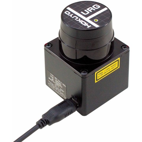
Hokuyo URG-04LX-UG01
Briefly about the principle of the laser scanner:
The range finder emits rays along the plane. The beam, which met an obstacle in its path, is reflected from it and comes back. From the phase difference between the signals sent and received, it is possible to judge how far the obstacle is located.
Accordingly, if the emitted beam did not return, then at 5–6 meters along its direct emission or there are no obstacles, or the beam could not correctly reflect.

The following data can be obtained from the laser scanner:
For each emitted beam:
* Each of the parameters is stored in a separate array and corresponds to the data for one of the rays.
To map the map and draw it, I used the ROS (Robot Operating System) tools, namely: the Rviz program and the data type nav_msgs :: OccupancyGrid. I created a publisher of a local map with the message type nav_msgs :: OccupancyGrid under the relevant topic local_map. In Rviz, subscribing to this topic, took the data about the map and displayed them in the form of the type Map.
In accordance with this algorithm, it was necessary to programmatically adjust the processing of data from the laser scanner and record them in the required format for transmission. In OccupancyGrid, the map is stored and transmitted in a one-dimensional array.
Appeal to any element of such a one-dimensional array is as follows:
mapSize — local map size
j — column number
i — row number
Map cells (again, according to the OccupancyGrid data type) should have values from 0 to 100. The smaller the value, the greater the likelihood that the cell is passable and vice versa.
To simplify the task, I selected 3 primary colors for cell coloring.
An important point!
Before the arrival of data from the scanner, the map is completely unknown (the values of all cells = 50) and each time after drawing, it is again updated to an unknown state. This is done so that the map does not overlap with itself the extra, previous values. After all, the local map reflects the state of the environment only at a given time.
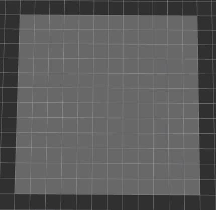
Unknown Map
Rays are constructed using a transformation from the polar coordinate system (UCS)
to the Cartesian coordinate system (DSC).
x, y - new coordinates in DSC
r - distance to obstacle
φ - the angle by which the beam
r was rejected , φ - old coordinates in the UCS
Fully pass through arrays of distances r and angles φ of rays (UCS data). For each item, do the following:

The simplest example of how a walkable path to an obstacle is built
Finally, the final touches!
Each card has permission. Simply put, this is the number of cells that can fit in 1 cell.
For example,
if there is 1 cell in 1 cell (the simplest case), then the resolution is 1.
If there is 5 cells in 1 cell, then the resolution is 0.2.
The resolution of my card is 0.04. That is, there are 25 cells in each cell. Thus, my minimum step is 4 cm. And 1 cell is 1m.
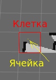
The difference of cells and cells on my map
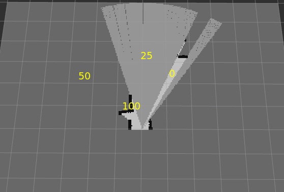
An example of building a local cross-country map
* Yellow colors indicate cell colors.
I believe that in general, the work I have done was successful, but I understand that the algorithm is imperfect and requires clarification and refinement.
In this publication I would like to talk about how I built a local map of patency for the robot. This task was necessary both to improve the skills in programming and mastering sensors, and for the subsequent introduction of our own algorithms into the work of real robots at such robotic activities such as Robocross and Robofest.
This article is designed for those who are just entering the world of robotics or trying to figure out how to build a terrain map. I tried to present everything in the simplest and most understandable language that most people can understand.
What is a local card terrain
So, the local cross - country map is what the robot sees at a given time.
This is the information that comes from the “eye” of the robot and is subsequently processed and displayed in a convenient form.
If the robot is standing still, its local map under constant environmental conditions remains constant.
If the robot moves, then at any given time its environment is different, respectively, the local map also changes.
A local map usually has a fixed size. The size is calculated based on the maximum length of the beams emitted by the rangefinder. In my case, this length is 6 meters.
To simplify the task for itself, it was decided to make a square map. It was also decided that the range finder would be conventionally located exactly in the center of the map (this place would be the point where x = y = 0). The center was chosen in this way because the range finder that I use emits rays in the plane of more than 180 ° (it emits rays at 240 °, but more on that later), that is, some rays will certainly go beyond the scanner and if you choose the wrong center, you can lose them. With proper center selection, all rays will be correctly displayed. On this basis, the size of the map I made is 2 times larger than the maximum length of the emitted rays.
The size of my card is 12 * 12 meters.
The sensor I used
In fact, to solve this kind of problem, you can use any rangefinder.
A range finder is a device for determining the distance to something (in my case to a potential obstacle).
In robotics, mainly 2 types of rangefinders are used: ultrasonic and laser.
Ultrasonic range finders are much cheaper, but ultrasonic beams are wide enough and are not suitable for accurate measurements.
Laser rangefinders are more expensive, but more precisely, since their rays are narrowly directed.
To solve my problem, I used the Hokuyo URG-04LX-UG01 laser scanner. This sensor is capable of emitting beams at 240 ° and gives fairly accurate information about the obstacles that are in the way of the beams. Its maximum range is 5-6 meters. It should be noted that this rangefinder emits rays only in a 2D plane. This fact obliges to put the sensor on the robot in a certain place, usually in front of the bottom of the robot, to get a more accurate picture. Again, you can use 3D scanners, which provide much more accurate and complete information about the environment, but they cost much more.
I believe that this particular scanner is perfect for training in the price-quality ratio.
Hokuyo URG-04LX-UG01
Briefly about the principle of the laser scanner:
The range finder emits rays along the plane. The beam, which met an obstacle in its path, is reflected from it and comes back. From the phase difference between the signals sent and received, it is possible to judge how far the obstacle is located.
Accordingly, if the emitted beam did not return, then at 5–6 meters along its direct emission or there are no obstacles, or the beam could not correctly reflect.
The following data can be obtained from the laser scanner:
For each emitted beam:
- Distance to obstacles
- Emission angle
* Each of the parameters is stored in a separate array and corresponds to the data for one of the rays.
About building a map
To map the map and draw it, I used the ROS (Robot Operating System) tools, namely: the Rviz program and the data type nav_msgs :: OccupancyGrid. I created a publisher of a local map with the message type nav_msgs :: OccupancyGrid under the relevant topic local_map. In Rviz, subscribing to this topic, took the data about the map and displayed them in the form of the type Map.
In accordance with this algorithm, it was necessary to programmatically adjust the processing of data from the laser scanner and record them in the required format for transmission. In OccupancyGrid, the map is stored and transmitted in a one-dimensional array.
What's going on here?
Для тех, кто впервые сталкивается с подобным типом данных ROS: это необычно, так как карта привычным образом представяется в виде двумерного массива с определенным числом столбцов и строк.
Так было и у меня. Карту на основе данных со сканера я храню в двумерном массиве, а при формировании сообщения для отправки в Rviz, я преобразую двумерный массив в одомерный, необходимый для OccupancyGrid.
На самом деле карта в OccupancyGrid только хранится и передается в одномерном массиве. При расшифровке ее данных она автоматически превратится в квадратную двумерную карту.
Но чтобы это произошло корректно, необходимо записывать этот одномерный масив определенным образом.
А именно: строчка за строчкой из двумерного хранилища записывать в одну строку.
Вуаля! Это весь секрет.
Appeal to any element of such a one-dimensional array is as follows:
l o c a l M a p [ m a p S i z e ∗ j + i ]
mapSize — local map size
j — column number
i — row number
Map cells (again, according to the OccupancyGrid data type) should have values from 0 to 100. The smaller the value, the greater the likelihood that the cell is passable and vice versa.
To simplify the task, I selected 3 primary colors for cell coloring.
- White - passable zone = 0
- Black - impassable zone = 100
- Gray - unknown zone = 50
An important point!
Before the arrival of data from the scanner, the map is completely unknown (the values of all cells = 50) and each time after drawing, it is again updated to an unknown state. This is done so that the map does not overlap with itself the extra, previous values. After all, the local map reflects the state of the environment only at a given time.
Unknown Map
Rays are constructed using a transformation from the polar coordinate system (UCS)
to the Cartesian coordinate system (DSC).
x, y - new coordinates in DSC
r - distance to obstacle
φ - the angle by which the beam
r was rejected , φ - old coordinates in the UCS
Algorithm of data processing from the sensor:
Fully pass through arrays of distances r and angles φ of rays (UCS data). For each item, do the following:
- Transform the coordinates from the PSK to the DSC for the final r and φ. Paint the resulting cell black. This is an obstacle.
- We pass in a straight line from the location of the scanner to the cell with an obstacle with a certain step, in the simplest case equal to the size of the cell.
- Again, convert the data from the PSK to the DSC and paint the new cell in white. This is a passable zone.
The simplest example of how a walkable path to an obstacle is built
And what if the emitted beam did not return?
Если такое произошло, это может означать следующее:
*«Потеряться» луч может обычно потому, что отразился не под углом 180° (то есть под любым, который не дойдет обратно), так как препятствие могло стоять неперпендикулярно лучу. А как известно еще из физики: угол падения равен углу отражения.

Или потому, что препятствие было слишком черным и забрало в себя большую часть энергии луча и лучу не хватило энергии, чтобы вернуться обратно.
Таким образом, невозможно быть полностью уверенным в том, что произошло, если луч не вернулся.
Что делать в подобных ситуациях?
Делаем следующее:
Мы ничего не теряем, если лучи дейтвительно не встретили препятствий, а если какое-то препятствие все-таки ускользнуло от «глаз» робота, то оно обязательно обнаружится очень быстро.
- Луч «потерялся», то есть отразился не полностью или отразился в другом направлении
- На пути луча не возникло никаких препятствий и из-за этого ему просто не от чего было отражаться
*«Потеряться» луч может обычно потому, что отразился не под углом 180° (то есть под любым, который не дойдет обратно), так как препятствие могло стоять неперпендикулярно лучу. А как известно еще из физики: угол падения равен углу отражения.
Или потому, что препятствие было слишком черным и забрало в себя большую часть энергии луча и лучу не хватило энергии, чтобы вернуться обратно.
Таким образом, невозможно быть полностью уверенным в том, что произошло, если луч не вернулся.
Что делать в подобных ситуациях?
Делаем следующее:
- Считаем расстояние до препятствия такого луча максимально возможным для сканера (в нашем случае это 6 метров)
- Считаем все ячейки по прямой до препятствия полупроходимыми и присваиваем им промежуточное число 25. Это проходимые ячейки, но в них мы не до конца уверены.
Мы ничего не теряем, если лучи дейтвительно не встретили препятствий, а если какое-то препятствие все-таки ускользнуло от «глаз» робота, то оно обязательно обнаружится очень быстро.
Card resolution
Finally, the final touches!
Each card has permission. Simply put, this is the number of cells that can fit in 1 cell.
For example,
if there is 1 cell in 1 cell (the simplest case), then the resolution is 1.
If there is 5 cells in 1 cell, then the resolution is 0.2.
The resolution of my card is 0.04. That is, there are 25 cells in each cell. Thus, my minimum step is 4 cm. And 1 cell is 1m.
The difference of cells and cells on my map
What was the result?
An example of building a local cross-country map
* Yellow colors indicate cell colors.
I believe that in general, the work I have done was successful, but I understand that the algorithm is imperfect and requires clarification and refinement.