Creating a bot for participation in the AI mini cup 2018 based on a recurrent neural network (part 2)
- Tutorial

This is a continuation of the first part of the article.
In the first part of the article, the author spoke about the conditions of the competition for the game Agario on mail.ru, the structure of the game world and partly about the bot device. Partially, because they affected only the device of input sensors and commands at the exit from the neural network (further in pictures and text there will be an abbreviation NN). So try to open the black box and understand how everything is arranged there.
Here is the first picture:
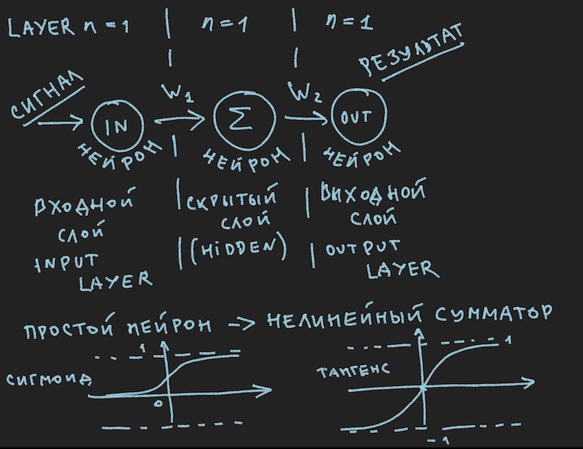
It schematically depicts something that should cause a bored smile to my reader, they say, again in first grade, they have seen it many times in various sources . But we want to practically apply this picture to the control of the bot, so after an Important Note, let’s look at it closely.
Important note: there are a large number of ready-made solutions (frameworks) for working with neural networks:

All these packages solve the main tasks for the developer of neural networks: the construction and training of NN or the search for "optimal" weights. And the main method of this search . Back Propagation Error (eng. Backpropagation). They invented it in the 70s of the last century, as indicated by the article at the above link, during this time, like the bottom of a ship, it was overgrown with various improvements, but the essence is the same: finding weights with a database of examples for training and it is highly desirable that of these examples contained a ready-made response in the form of the output signal of a neural network. I can argue the reader. that self-learning networks of various classes and principles have already been invented, but everything is not smooth there, as far as I understand. Of course, there are plans to explore this zoo in more detail, but I think I will find like-minded people in that a bicycle made by hand without any special drawings, even the most curved one is closer to the heart of the creator than the conveyor clone of an ideal bicycle.
Understanding that the game server most likely will not have these libraries and the computational power allocated by the organizers in the form of 1 processor core is clearly not enough for a heavy framework, the author went by creating his own bike. An important note is over.
Let us return to the picture depicting probably the simplest possible neural networks with a hidden layer (also known as the hidden leer or hidden layer). Now the author himself has closely looked at the picture with ideas on this simple example to slightly open up to the reader the depths of artificial neural networks. When everything is simplified to a primitive, it is easier to understand the essence. The bottom line is that a hidden layer of a hidden layer has nothing to add. And most likely it is not even a neural network; in the textbooks, the simplest NN is a network with two inputs. So here we are, as it were, the discoverers of the simplest of the simplest networks.
Let's try to describe this neural network (pseudocode):
We introduce a network topology in the form of an array, where each element corresponds to the layer and the number of neurons in it:
int array Topology= { 1, 1, 1}
We also need a float array of weights of the W neural network, considering our network as a “forward neural networks, FF or FFNN” neural network, where each neuron of the current layer is connected to each neuron of the next layer, we obtain the dimension of the array W [number of layers , the number of neurons in the layer, the number of neurons in the layer]. Not quite the optimal encoding, but given the GPU hot breath somewhere very close in the text, it is understandable.
A short procedure for CalculateSize counting the number of neurons neuroncountand the number of their connections in a neural network dendritecount, I think will explain better the author’s nature of these connections:
voidCalculateSize(arrayint Topology,  int neuroncount, int dendritecount){
 for (int i : Topology)  // i идет по лейерам и суммирует нейроны всех слоев
        neuroncount += i;
    for (int layer = 0, layer <Topology.Length - 1, layer++) //идет по лейерамfor (int i = 0, i < Topology[layer] + 1, i++)        //идет по нейронам for (int j = 0, j < Topology[layer + 1], j++)   //идет по нейронам
                dendritecount++;
}
My reader, the one who already knows all this, the author came to such an opinion in the first article, of course, he wondered why in the third nested cycle Topology [layer1 + 1] instead of Topology [layer1], which gives the neuron more than in the network topology . And I will not answer. It is also useful for the reader to set tasks at home.
We are almost a step away from building a working neural network. It remains to add the function of summing signals at the input of the neuron and its activation. There are many activation functions, but those closest to the nature of the neuron are Sigmoid and Tangensoid (probably it is better to call it this, although this name is not particularly used in the literature, the maximum of the tangensoid, but this is the name of the graph, but what is a graph if not a reflection of the function?)
So we have the neuron activation functions (in the picture they are present, in its lower part)
float Sigmoid(float x)
{
    if (x < -10.0f) return0.0f;
    elseif (x > 10.0f) return1.0f;
    return (float)(1.0f / (1.0f + expf(-x)));
}
Sigmoid returns values from 0 to 1.
floatTanh(float x)
{
    if (x < -10.0f) return-1.0f;
    elseif (x > 10.0f) return1.0f;
    return (float)(tanhf(x));
}
Tangensoid returns values from -1 to 1.
The basic idea of the signal passing through the neural network is a wave: a signal is sent to the input neurons-> through neural connections; the signal passes to the second layer-> the neurons of the second layer sum up the signals that have reached them, modified by interneuron weights-> added through the additional weight bias (bias) -> We use the activation-> function and go to the next layer (read the first cycle of the example from the layers), that is, from the very beginning, this repetition of the chain will be the neurons of the next layer. In simplification, it is not even necessary to store the values of the neurons of the entire network; you only need to store the weights NN and the values of the neurons of the active layer.
Once again, we give a signal to the input NN, the wave ran through the layers and remove the obtained value on the output layer.
Here, it is possible to programmatically solve the reader's taste with the help of recursion or just a triple cycle as the author has, in order to speed up the calculations it is not necessary to fence objects in the form of neurons and their connections and other OOP. Again, this is connected with the sensation of close GPU calculations, and on graphics processors, due to their nature of mass parallelism, OOP is a little stuck, this is relative to the languages c # and c ++.
Next, I propose that the reader independently go through the path of building a neural network in the code, with his reader having a voluntary desire, the absence of which is quite understandable and familiar to the author, as for examples of building NN from scratch, there are a large number of examples in the network, so it will be difficult to go astray as straightforward as a neural network of direct distribution in the above picture.
But where the new pictures exclaim the reader, who has not yet departed from the previous passage, and will be right, in childhood the author determined the value of the book from illustrations to it. Here you are:
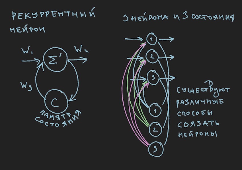
In the picture we see a recurrent neuron and the NN constructed from such neurons is called recurrent or RNN. This neural network has a short-term memory and is chosen by the author for the bot as the most promising from the point of view of adaptation to the game process. Of course, the author built a direct distribution neural network, but in the process of searching for an “effective” solution, he switched to RNN.
The recurrent neuron has an additional state C, which is formed after the first passage of the signal through the neuron, Tick + 0 on the time scale. In simple terms, this is a copy of the output signal of the neuron. In the second step, read Tick + 1 (since the network operates at the frequency of the gaming bot and server), the value C returns to the input of the neural layer through additional weights and thus participates in the formation of the signal, but by Tick + 1 time.
Note: in research groups' work on controlling NN gaming bots , there is a tendency to use two rhythms for a neural network, one rhythm is the frequency of a game Tic, the second rhythm, for example, is two times slower than the first. Different parts of NN operate at different frequencies, which gives a different vision of the game situation inside the NN, thereby increasing its flexibility.
To build the RNN in the bot code, we introduce into the topology an additional array, where each element corresponds to a layer and the number of neural states in it:
int array TopologyNN= { numberofSensors, 16, 8, 4}int array TopologyRNN= { 0, 16, 0, 0 }
From the above topology, it is clear that the second layer is recurrent, since it contains neural states. We also introduce additional weights in the form of a float of the WRR array, the same dimension as the W array.
The counting of connections in our neural network will change slightly:
for (int layer = 0, layer < TopologyNN.Length - 1, layer++)
    for (int i = 0, i  < TopologyNN[layer] + 1, i++)
         for (int j = 0, j <  TopologyNN[layer + 1] , j++)
                dendritecount++;
 for (int layer = 0, layer < TopologyRNN.Length - 1, layer++)
       for (int i = 0, i< TopologyRNN[layer] + 1 , i++)
            for (int j = 0, j< TopologyRNN[layer],  j++)
                dendritecount++;
The author will attach the general code of the recurrent neural network at the end of this article, but the main thing here is to understand the principle: passing waves through layers in the case of recurrent NN does not fundamentally change anything, only one more term is added to the neuron activation function. This is the term of the state of neurons on the previous Tick multiplied by the weight of neural communication.
We will assume that they have refreshed the theory and practice of neural networks, but the author clearly realizes that he did not bring the reader closer to understanding how to train this simple structure of neural connections to make any decisions in the game process. We don’t have libraries with examples for teaching NN. In the Internet groups of developers of bots, the opinion sounded: give us a log file in the form of coordinates of bots and other game information for the formation of a library of examples. But the author unfortunately could not figure out how to use this log file for learning NN. I will be glad to discuss this in the comments to the article. Therefore, the only available for the author's understanding of the method of learning, or rather the finding of "effective" neural weights (neural links), was the genetic algorithm.
A picture was prepared about the principles of the genetic algorithm:
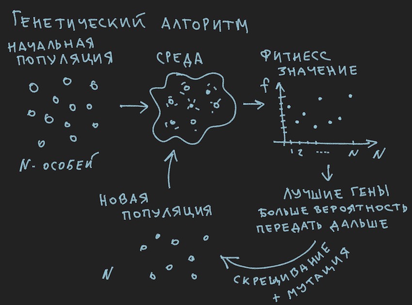
So the genetic algorithm .
The author will try not to delve into the theory of this process , but to recall only the minimum necessary to continue the full reading of the article.
In the genetic algorithm, the main working body is the gene (DNA is the name of the molecule). In our case, the genome is a sequential set of genes or a one-dimensional array of float long ...
At the initial stage of work with only the built neural network, it is necessary to initialize it. Initialization is the assignment of random values from -1 to 1 to the neural weights. The author mentioned that the range of values from -1 to 1 is too extreme and the trained networks have weights in a smaller range, for example, from -0.5 to 0.5, and that the initial range of values should be different. from -1 to 1. But we will go classic by collecting all the difficulties in one gate and take the widest possible segment of the initial random variables as the basis for the initialization of the neural network.
Now there will be a bijection . We will assume that the length (size) of a bot's genome will be equal to the total length of the neural network arrays TopologyNN.Length + TopologyRNN.Length it’s not for nothing that the author spent the reader’s time on the neural link counting procedure.
Note: As the reader has already noted for himself, we transfer only the weights of the neural network to the genotype, the structure of connections, activation functions, and the state of neurons are not transferred. For a genetic algorithm, only neural connections are sufficient, which suggests that they are the information carriers. There are developments where the genetic algorithm also changes the structure of connections in the neural network and is fairly easy to implement. Here, the author leaves the space for creativity to the reader, although he himself will think about it with interest: you need to understand to use two independent genomes and two fitness functions (simply two independent genetic algorithms) or you can all under one genome and algorithm.
And since we initialized NN with random variables, we thereby initialized the genome. The reverse process is also possible: initialization of the genotype with random variables and its subsequent copying into neural weights. The usual is the second option. Since the genetic algorithm in the program often exists separately from the entity itself and is associated with it only by the genome data and the value of the fitness function ... Stop, stop, the reader will say, the population clearly shows in the picture and not a word about a single genome.
Well, add pictures to the oven of the reader's mind:
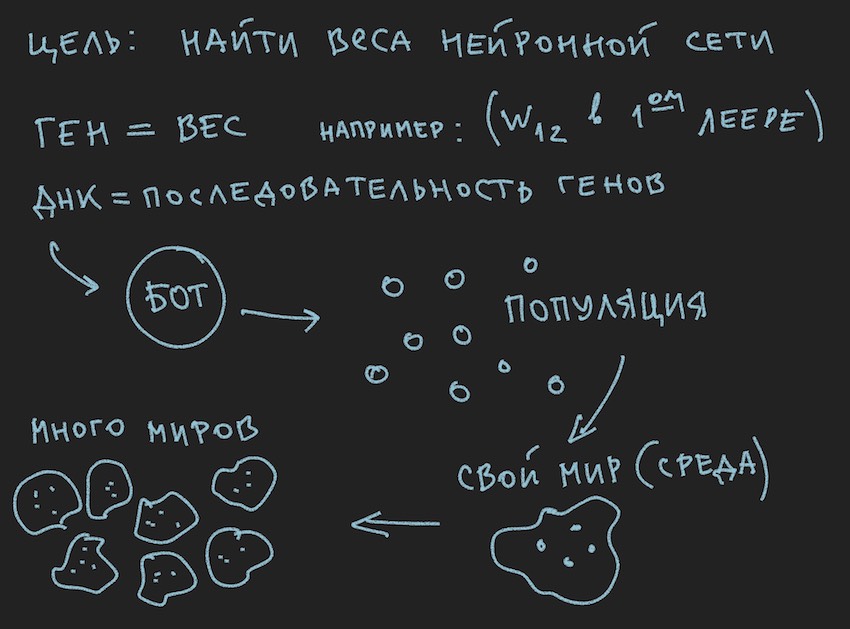
Since the author drew the pictures before writing the text of the article, they support the text, but do not follow the letter to the letter of the current narration.
From the drawn information it follows that the main working body of the genetic algorithm is the population of genomes . This is a bit contrary to what was previously said by the author, but how to do in the real world without minor contradictions. Yesterday the sun rotated around the earth, and today the author talks about a neural network inside a software bot. No wonder he baked the mind remembered.
I trust the reader to understand the question about the contradictions of the world. The bot world is quite self-sufficient for the article.
But what the author has already done, to this part of the article, is to form a population of bots.
Let's look at it from the program side:
There is a bot (it can be an object in the OOP, a structure, although this is probably also an object or just an array of data). Inside, the bot contains information about its coordinates, speed, mass, and other information useful in the gameplay, but the main thing for us now is that it contains a link to its own genotype or the genotype itself, depending on the implementation. Then you can go in different ways, limit yourself to arrays of the neural network weights, or enter an additional array of genotypes, as it will be convenient for the reader to imagine in your imagination. At the first stages, the author selected arrays of neural weights and genotypes in the program. Then he refused to duplicate information and limited himself to the weights of the neural network.
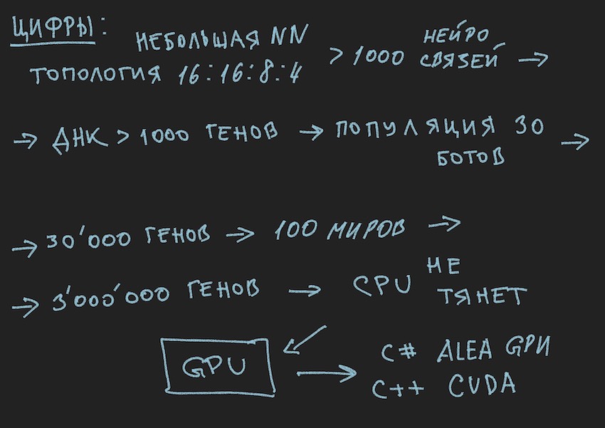
Following the logic of the story you need to tell that the population of bots is an array of the above bots. What is the game cycle ... Stop again, what game cycle? the developers politely provided only one place for Bot to board the game simulation program on the server or a maximum of four bots in the local simulator. And if you recall the topology of the neural network chosen by the author:
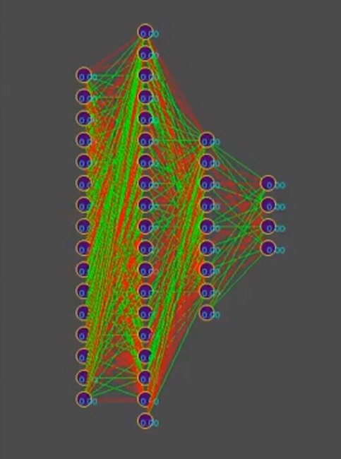
And suppose, to simplify the narration, that the genotype contains about 1000 neural connections, by the way, in the simulator, the genotypes look like this (the red color is the negative value of the gene, the green is the positive value, each line is a separate genome):
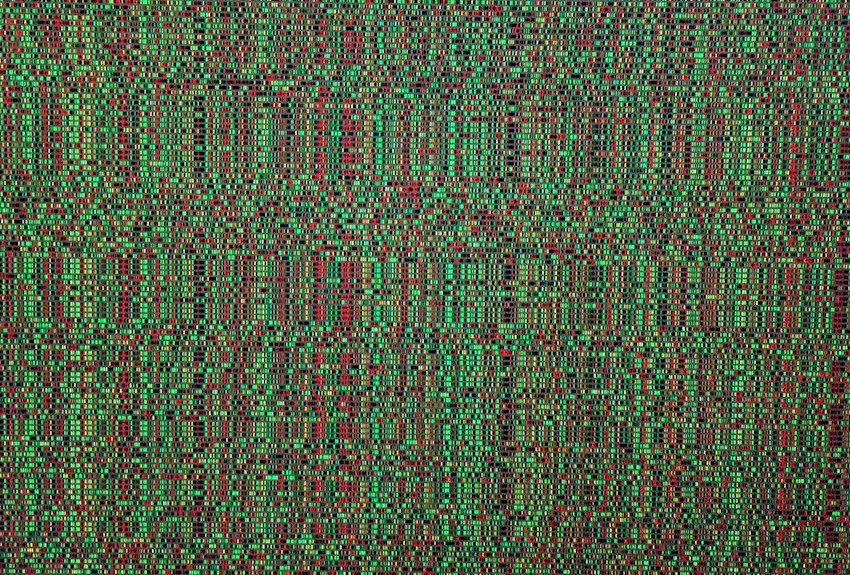
Note to the photo: over time, the pattern changes towards the dominance of one of the solutions; vertical bars are common genes of genotypes.
So, we have 1000 genes in the genotype and a maximum of four bots in the simulator program of the game world from the organizers of the competition. How many times it is necessary to run the simulation of the battle of bots in order to bust, even the cleverest, to come closer in search to the "effective"
genotype, read the "effective" combination of neural connections, provided that each neural connection varies from -1 to 1 in increments, and which step? initialization was random float, it is 15 decimal places. Step is not yet clear to us. On the number of variants of neural weights, the author assumes that this is an infinite number, when choosing a certain step size, probably a finite number, but in any case, these numbers are much more than 4 places in the simulator, even considering the sequential launch from the queue of bots plus simultaneous parallel launch of official simulators, up to 10 on one computer (for fans of vintage programming: a computer).
I hope the pictures help the reader.
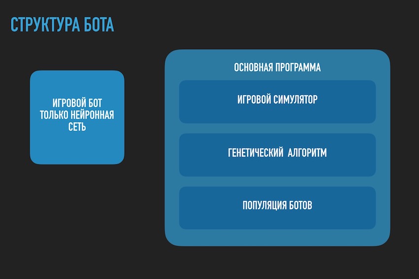
Here you need to pause and talk about the architecture of the software solution. Since the solution in the form of a separate software bot downloaded to the competition site is no longer suitable. It was necessary to divide the bot playing according to the rules of the competition within the framework of the ecosystem of the organizers and the program trying to find a neural network configuration for it. The diagram below is taken from the conference presentation, but generally reflects the real picture.
Remembered the bearded anecdote:
Large organization.
Time is 18.00, all employees work as one. Suddenly one of the employees turns off the computer, gets dressed and leaves.
All escorted him with a surprised look.
The next day. At 18.00 the same employee turns off the computer and leaves. Everyone continues to work and begin to whisper with displeasure.
The next day. At 18.00, the same employee turns off the computer ...
A colleague comes up to him:
-How do not you feel ashamed, we are working, the end of the quarter, so many reports, we also want to go home on time and you are such a one-man ...
-Guys, yes, I generally have a VACATION!
… to be continued.
Yes, I almost forgot to attach the code for the RNN calculation procedure, it is valid and written independently, so maybe there are errors in it. To enhance, I will bring it as it is, it is in c ++ with reference to CUDA (library for calculating on the GPU).
Note: multi-dimensional arrays do not get along well on GPUs, there are of course textures and matrix calculations, but it is recommended to use one-dimensional arrays.
An example of an array [i, j] of dimension M along j becomes an array of the form [i * M + j].
__global__ void cudaRNN(Bot *bot, argumentsRNN *RNN, ConstantStruct *Const, int *Topology, int *TopologyRNN, int numElements, int gameTick)
{
    int  tid = blockIdx.x * blockDim.x + threadIdx.x;
    int  threadN = gridDim.x * blockDim.x;
    int TopologySize = Const->TopologySize;
    for (int pos = tid; pos < numElements; pos += threadN)
    {
        const  int ii = pos;
        const int iiA = pos*Const->ArrayDim;
        int ArrayDim = Const->ArrayDim;
        const int iiAT = ii*TopologySize*ArrayDim;
        if (bot[pos].TTF != 0 && bot[pos].Mass>0)
        {
            RNN->outputs[iiA + Topology[0]] = 1.f;  //bias
            int neuroncount7 = Topology[0];
            neuroncount7++;
            for (int layer1 = 0; layer1 < TopologySize - 1; layer1++)
            {
                for (int j4 = 0; j4 < Topology[layer1 + 1]; j4++)
                {
                    for (int i5 = 0; i5 < Topology[layer1] + 1; i5++)
                    {
                        RNN->sums[iiA + j4] = RNN->sums[iiA + j4] + RNN->outputs[iiA + i5] *
                            RNN->NNweights[((ii*TopologySize + layer1)*ArrayDim + i5)*ArrayDim + j4];
                    }
                }
                if (TopologyRNN[layer1] > 0)
                {
                    for (int j14 = 0; j14 < Topology[layer1]; j14++)
                    {
                        for (int i15 = 0; i15 < Topology[layer1]; i15++)
                        {
                            RNN->sumsContext[iiA + j14] = RNN->sumsContext[iiA + j14] +
                                RNN->neuronContext[iiAT + ArrayDim * layer1 + i15] *
                                RNN->MNweights[((ii*TopologySize + layer1)*ArrayDim + i15)*ArrayDim + j14];
                        }
                        RNN->sumsContext[iiA + j14] = RNN->sumsContext[iiA + j14] + 1.0f*
                            RNN->MNweights[((ii*TopologySize + layer1)*ArrayDim + Topology[layer1])*ArrayDim + j14]; //bias=1
                    }
                    for (int t = 0; t < Topology[layer1 + 1]; t++)
                    {
                        RNN->outputs[iiA + t] = Tanh(RNN->sums[iiA + t] + RNN->sumsContext[iiA + t]);
                        RNN->neuronContext[iiAT + ArrayDim * layer1 + t] = RNN->outputs[iiA + t];
                    }
                    //SoftMax/*
                    double sum = 0.0;
                    for (int k = 0; k <ArrayDim; ++k)
                        sum += exp(RNN->outputs[iiA + k]);
                    for (int k = 0; k < ArrayDim; ++k)
                        RNN->outputs[iiA + k] = exp(RNN->outputs[iiA + k]) / sum;
*/
                }
                else
                {
                    for (int i1 = 0; i1 < Topology[layer1 + 1]; i1++)
                    {
                        RNN->outputs[iiA + i1] = Sigmoid(RNN->sums[iiA + i1]); //sigma
                    }
                }
                if (layer1 + 1 != TopologySize - 1)
                {
                    RNN->outputs[iiA + Topology[layer1 + 1]] = 1.f;
                }
                for (int i2 = 0; i2 < ArrayDim; i2++)
                {
                    RNN->sums[iiA + i2] = 0.f;
                    RNN->sumsContext[iiA + i2] = 0.f;
                }
            }
        }
    }
}