Boring Integrals
Some of you probably saw this problem on the open spaces of the network: what number continues the next row?
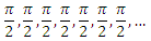
Such an obvious correct answer was proposed:

For those who did not understand how it was obtained, an explanation was offered. Let (well, 1 for x = 0, although it does not matter). Then each member of the series is the value of the following integral in the chain:
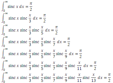
So far, everything is going well, but then suddenly:

In principle, this is enough to amuse mathematician friends, but I wanted to find out how such integrals are generally considered and why such a ridiculous result is obtained. If someone else wants to shake the old days and remember the matan with the funkan, please read on.
First, let's take a look at the first integral separately:

Some time ago, I thought: “Hey, I haven't completely forgotten the matan! Let me take this integral as indefinite, and then set the limits. Surely a couple of times in parts, and the thing is in the hat. Now I’ll decide on a piece of paper without outside help. ” I want to warn you: do not repeat my mistake. A sleepless night awaits you, and then you look in the directory and find out that the indefinite integral is not taken in elementary functions. For him, they even introduced a special function .
However, with these specific limits, the integral can be taken in different ways. We will go in a way that requires a minimum of basic knowledge (the most severe is the same integration in parts). To start, we will make a sudden replacement:
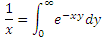
You ask: where did this come from and why do we need another integral, is it not enough? It’s calm, it’s necessary (those familiar with the properties of the Laplace transform are grinning cheerfully). We substitute the replacement in the original formula and change the order of integration:

Inside, we got an almost classical integral over dx , which scared everyone in our physics school. It can also be taken as indefinite, using the integration formula in parts twice. Then on the right we get some kind of turbidity and once again the same integral multiplied by something, and as a result it will be possible to solve the equation for this integral and get an answer, and then set the limits. Who cares, do it yourself, and I will lazily write down the finished result:

Well, now everything is simple: this is a table integral from a secondary school, which is equal to the arc tangent. At infinity, in half, at zero - zero, so we got the answer.
The integral, by the way, is so good that it has its own name - the Dirichlet integral . From the link you can find other ways to take it.
For the next trip, we need four things: a rectangular function, a cosine Fourier transform, convolution, and Parseval's theorem. First, I’ll say a few words about these wonderful things.
A rectangular function - we will have such a step around zero:

The value 1/2 at the points of discontinuity is necessary mainly for observing the properties of the Fourier transform, as a whole it is unprincipled for our task.
Cosine Fourier Transform . For simplicity, we digress a little from mathematical accuracy and formulate it roughly. For a sufficiently good even function f (x), the following relations hold:
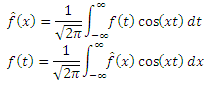
Function and is called the cosine Fourier transform (FCT) of f (x) (it is also called the image of f). That is, the cosine transform from the cosine transform gives again the original function f (x)!
People familiar with signal processing are well aware that FCT from a rectangular function is this . This is easy to prove using the above formulas and school knowledge. Since the rectangular function outside the interval [-a, a] is equal to zero, we can simply integrate cos (xt) dt over this interval, here we can simply replace the variable and the table integral. The property above says that FCT from is a rectangular function.
Convolution is another great thing that signal processing can do without. For two functions f 1 (x) and f 2(x) you can define the convolution function (indicated by an asterisk) like this:

The convolution has a wonderful property for which it is loved: the Fourier transform turns it into multiplication, and multiplication into convolution. More specifically, the product of two cosine transform good of even functions is the convolution of their images, divided by the square root of two pi: .
.
Parseval's theorem is a very cool statement about the equality of the signal energy and its spectrum, which is written differently for different purposes. We need this version: for even and fairly good functions .
.
Take the second integral from our wonderful sequence. As many have already guessed, we will use Parseval's theorem and replace the factors with their FCT-images:

The first rectangular function under the integral is equal to one for arguments less than one and zero for arguments more than one. Therefore, nothing prevents us from removing it from the integral by adjusting the limits of integration:

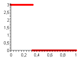
Under the integral there is a step with a height of 3 and a width of 1/3. Even a third grader will take such an integral: you just need to multiply 3 and 1/3. One remains from the integral, and we have the desired pi in half! Thus, we almost honestly took the second integral from the series. Those who wish to do this quite honestly will have to figure out what the goodness of a function is and prove that our functions are good.
To make things easier later, we designate this step under the integral as F 1 (x) and draw its graph:
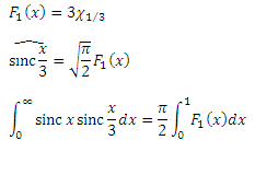
Let's go on having fun and look at the integral with three factors. To apply the theorem of Parseval, we are now all the factors in the second we shall consider one factor: . With the image of the first factor, everything is already clear, and the image of the second factor is expressed through convolution:

At first glance it’s creepy. But you can raise something, cut something and substitute our F 1 (x) . Then we get: The

internal integral is just a rectangular filter, a kind of “bluer” for the function F 1 (x): we simply average for each point all values in the neighborhood plus or minus one fifth. Again, you can get rid of the rectangular function by poking the limits of integration. And with the external integral we will do the same procedure. Here is the result:

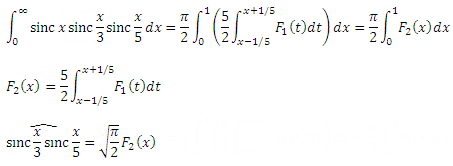
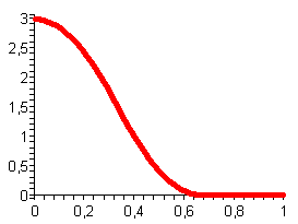
On the left is the graph of the function F 2 (x) , which is actually a smoothed F 1 (x). It is easy to prove that after smoothing a function along a normalized kernel, its integral does not change. Well, actually we are talking about the integral from -∞ to + ∞, but for an even function this is also true for an integral from zero. In this case, the kernel was a step from -1/5 to +1/5, multiplied by 5/2. The area under the step is unity, which means that the core is normalized. Here, too, you can compare with the bluer in Photoshop: after applying the blue, the picture as a whole does not become lighter or darker. And if so, then the integral F 2 (x) is exactly equal to the integral F 1 (x) , that is, one, therefore the third integral is equal to pi-halves!
Further, the procedure is much similar. Group the fourth integral as follows: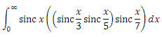 . First, the Parseval theorem, for the brackets is a convolution, and we already know how to express the image of the inner bracket in terms of F 2 (x) . Then everything is the same as last time, and as a result we get:
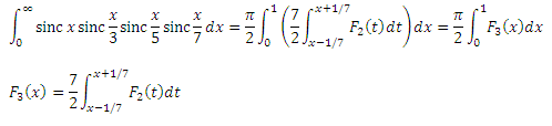
Now we already have F 3 (x) , which is actually a smooth F 2 (x) with a kernel 2/7 wide. The kernel is normalized, which means that the integral F 3 (x) is equal to the integral F 2 (x) , that is, one, and again we have pi-halves!
Great, we now click these integrals like nuts. But in theory, if it goes on like this, will they all be equal to infinity in half? Let's look further. Fifth integral:
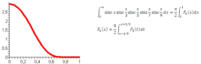
Everything seems to be the same. Okay, sixth integral:
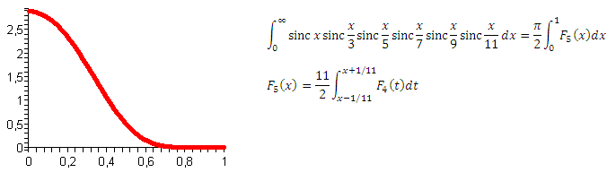
And there are no problems. Well, take the seventh:
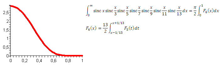
Nothing new! Okay, what about the eighth?
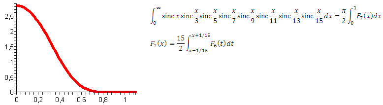
Stop stop stop! Here we can not do without the CSI team!

Function flowed through unit! The integral F 7 (x) is still equal to unity, but this is if we integrate from 0 to ∞. And we integrate to unity! Until now, all functions have been zero when x is greater than unity, but sooner or later it should have ended.
But how to understand when the end is coming? It is very simple. F 1 (x) was nonzero at x <1/3. F 2 (x)smoothed it by ± 1/5, which means that it was nonzero at x <1/3 + 1/5. In a similar way, one can find the boundary of nonzero values for all these functions, and for F 7 (x) this boundary exceeds unity for the first time:

It is easy to even calculate how much has leaked, and thereby calculate the exact value of the eighth integral. Note that to the left of the boundary F 1 (x) is a constant 3. F 2 (x) is minus the integral of this constant with a coefficient of 5/2, that is, a straight line with a coefficient of 3 × 5/2. F 3 (x) in sufficient proximity to the boundary 1/3 + 1/5 + 1/7 is the integral of that line with a coefficient of 7/2, that is, something like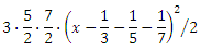 . Continuing similar reasoning, we obtain the formula for F 7 (x) in the vicinity of the boundary:

Actually, an ordinary parabola of the sixth degree, shifted and multiplied. If we integrate it from a unit to the border of 1/3 + 1/5 + 1/7 + 1/9 + 1/11 + 1/13 + 1/15, we will find out how many functions have leaked outside the unit. You can solve this problem entirely in ordinary fractions. The result is how much:

If we subtract this figure from unity and multiply by pi-half, we get the final value of the eighth integral:
Such integrals are called Borwain integralsin honor of David and Jonathan Borwein, who described them. If you want rigorous mathematical proofs (without any “good functions”) and other properties of these wonderful integrals, read the article by the authors .
Having opened these integrals, Jonathan Borvein introduced them into the Maple software package and, making sure that Maple correctly takes all eight integrals, he informed the developers about the “bug”: they say that the eighth integral should also be in half, and you get the hell what. Three days and three nights were killed by Jacques Carett , one of the developers of Maple, in search of a mistake, until he realized that he was cruelly joked. And they say that mathematicians are boring people!
Such an obvious correct answer was proposed:
For those who did not understand how it was obtained, an explanation was offered. Let
(well, 1 for x = 0, although it does not matter). Then each member of the series is the value of the following integral in the chain: So far, everything is going well, but then suddenly:
In principle, this is enough to amuse mathematician friends, but I wanted to find out how such integrals are generally considered and why such a ridiculous result is obtained. If someone else wants to shake the old days and remember the matan with the funkan, please read on.
A fairy tale begins to tell
First, let's take a look at the first integral separately:
Some time ago, I thought: “Hey, I haven't completely forgotten the matan! Let me take this integral as indefinite, and then set the limits. Surely a couple of times in parts, and the thing is in the hat. Now I’ll decide on a piece of paper without outside help. ” I want to warn you: do not repeat my mistake. A sleepless night awaits you, and then you look in the directory and find out that the indefinite integral is not taken in elementary functions. For him, they even introduced a special function .
However, with these specific limits, the integral can be taken in different ways. We will go in a way that requires a minimum of basic knowledge (the most severe is the same integration in parts). To start, we will make a sudden replacement:
You ask: where did this come from and why do we need another integral, is it not enough? It’s calm, it’s necessary (those familiar with the properties of the Laplace transform are grinning cheerfully). We substitute the replacement in the original formula and change the order of integration:
Inside, we got an almost classical integral over dx , which scared everyone in our physics school. It can also be taken as indefinite, using the integration formula in parts twice. Then on the right we get some kind of turbidity and once again the same integral multiplied by something, and as a result it will be possible to solve the equation for this integral and get an answer, and then set the limits. Who cares, do it yourself, and I will lazily write down the finished result:
Well, now everything is simple: this is a table integral from a secondary school, which is equal to the arc tangent. At infinity, in half, at zero - zero, so we got the answer.
The integral, by the way, is so good that it has its own name - the Dirichlet integral . From the link you can find other ways to take it.
Soon the fairy tale affects, but not soon the thing is done
For the next trip, we need four things: a rectangular function, a cosine Fourier transform, convolution, and Parseval's theorem. First, I’ll say a few words about these wonderful things.
A rectangular function - we will have such a step around zero:
The value 1/2 at the points of discontinuity is necessary mainly for observing the properties of the Fourier transform, as a whole it is unprincipled for our task.
Cosine Fourier Transform . For simplicity, we digress a little from mathematical accuracy and formulate it roughly. For a sufficiently good even function f (x), the following relations hold:
Function
and is called the cosine Fourier transform (FCT) of f (x) (it is also called the image of f). That is, the cosine transform from the cosine transform gives again the original function f (x)! People familiar with signal processing are well aware that FCT from a rectangular function is this
. This is easy to prove using the above formulas and school knowledge. Since the rectangular function outside the interval [-a, a] is equal to zero, we can simply integrate cos (xt) dt over this interval, here we can simply replace the variable and the table integral. The property above says that FCT from is a rectangular function. Convolution is another great thing that signal processing can do without. For two functions f 1 (x) and f 2(x) you can define the convolution function (indicated by an asterisk) like this:
The convolution has a wonderful property for which it is loved: the Fourier transform turns it into multiplication, and multiplication into convolution. More specifically, the product of two cosine transform good of even functions is the convolution of their images, divided by the square root of two pi:
. Parseval's theorem is a very cool statement about the equality of the signal energy and its spectrum, which is written differently for different purposes. We need this version: for even and fairly good functions
.Doseleva Makar was digging gardens, and now Makar is in the voivode
Take the second integral from our wonderful sequence. As many have already guessed, we will use Parseval's theorem and replace the factors with their FCT-images:
The first rectangular function under the integral is equal to one for arguments less than one and zero for arguments more than one. Therefore, nothing prevents us from removing it from the integral by adjusting the limits of integration:
Under the integral there is a step with a height of 3 and a width of 1/3. Even a third grader will take such an integral: you just need to multiply 3 and 1/3. One remains from the integral, and we have the desired pi in half! Thus, we almost honestly took the second integral from the series. Those who wish to do this quite honestly will have to figure out what the goodness of a function is and prove that our functions are good.
To make things easier later, we designate this step under the integral as F 1 (x) and draw its graph:
Let's go on having fun and look at the integral with three factors. To apply the theorem of Parseval, we are now all the factors in the second we shall consider one factor:
. With the image of the first factor, everything is already clear, and the image of the second factor is expressed through convolution: At first glance it’s creepy. But you can raise something, cut something and substitute our F 1 (x) . Then we get: The
internal integral is just a rectangular filter, a kind of “bluer” for the function F 1 (x): we simply average for each point all values in the neighborhood plus or minus one fifth. Again, you can get rid of the rectangular function by poking the limits of integration. And with the external integral we will do the same procedure. Here is the result:
On the left is the graph of the function F 2 (x) , which is actually a smoothed F 1 (x). It is easy to prove that after smoothing a function along a normalized kernel, its integral does not change. Well, actually we are talking about the integral from -∞ to + ∞, but for an even function this is also true for an integral from zero. In this case, the kernel was a step from -1/5 to +1/5, multiplied by 5/2. The area under the step is unity, which means that the core is normalized. Here, too, you can compare with the bluer in Photoshop: after applying the blue, the picture as a whole does not become lighter or darker. And if so, then the integral F 2 (x) is exactly equal to the integral F 1 (x) , that is, one, therefore the third integral is equal to pi-halves!
Further, the procedure is much similar. Group the fourth integral as follows:
. First, the Parseval theorem, for the brackets is a convolution, and we already know how to express the image of the inner bracket in terms of F 2 (x) . Then everything is the same as last time, and as a result we get: Now we already have F 3 (x) , which is actually a smooth F 2 (x) with a kernel 2/7 wide. The kernel is normalized, which means that the integral F 3 (x) is equal to the integral F 2 (x) , that is, one, and again we have pi-halves!
Great, we now click these integrals like nuts. But in theory, if it goes on like this, will they all be equal to infinity in half? Let's look further. Fifth integral:
Everything seems to be the same. Okay, sixth integral:
And there are no problems. Well, take the seventh:
Nothing new! Okay, what about the eighth?
Stop stop stop! Here we can not do without the CSI team!
Function flowed through unit! The integral F 7 (x) is still equal to unity, but this is if we integrate from 0 to ∞. And we integrate to unity! Until now, all functions have been zero when x is greater than unity, but sooner or later it should have ended.
But how to understand when the end is coming? It is very simple. F 1 (x) was nonzero at x <1/3. F 2 (x)smoothed it by ± 1/5, which means that it was nonzero at x <1/3 + 1/5. In a similar way, one can find the boundary of nonzero values for all these functions, and for F 7 (x) this boundary exceeds unity for the first time:
It is easy to even calculate how much has leaked, and thereby calculate the exact value of the eighth integral. Note that to the left of the boundary F 1 (x) is a constant 3. F 2 (x) is minus the integral of this constant with a coefficient of 5/2, that is, a straight line with a coefficient of 3 × 5/2. F 3 (x) in sufficient proximity to the boundary 1/3 + 1/5 + 1/7 is the integral of that line with a coefficient of 7/2, that is, something like
. Continuing similar reasoning, we obtain the formula for F 7 (x) in the vicinity of the boundary: Actually, an ordinary parabola of the sixth degree, shifted and multiplied. If we integrate it from a unit to the border of 1/3 + 1/5 + 1/7 + 1/9 + 1/11 + 1/13 + 1/15, we will find out how many functions have leaked outside the unit. You can solve this problem entirely in ordinary fractions. The result is how much:
If we subtract this figure from unity and multiply by pi-half, we get the final value of the eighth integral:
Such integrals are called Borwain integralsin honor of David and Jonathan Borwein, who described them. If you want rigorous mathematical proofs (without any “good functions”) and other properties of these wonderful integrals, read the article by the authors .
Conclusion: level eighty trolling
Having opened these integrals, Jonathan Borvein introduced them into the Maple software package and, making sure that Maple correctly takes all eight integrals, he informed the developers about the “bug”: they say that the eighth integral should also be in half, and you get the hell what. Three days and three nights were killed by Jacques Carett , one of the developers of Maple, in search of a mistake, until he realized that he was cruelly joked. And they say that mathematicians are boring people!