Introduction to Modular Arithmetic
In ordinary life, we usually use a positional number system. In a positional number system, the value of each numeric character (digit) in a number entry depends on its position (rank) [1]. However, there are so-called "non-positional number systems", one of which is the "residual class system" (RNS) (or the original Residue Number System (RNS)), which is the basis of modular arithmetic. Modular arithmetic is based on the "Chinese remainder theorem" [2], which for our case sounds as follows:
At first glance, it is not clear what advantage such a system can give, however, there are 2 properties that can effectively use modular arithmetic in some areas of microelectronics:
But not everything is as smooth as we would like. Unlike the positional number system, the following operations (called "non-modular") are more complicated than in the positional number system: comparing numbers, overflow control, division, square root, etc. The first successful attempts to use modular arithmetic in microelectronics were made back in the 1950s, but due to difficulties with non-modular operations, interest was somewhat abated. However, at present modular arithmetic is again returning to microelectronics for the following reasons:
Currently, modular arithmetic is used in the following areas: digital signal processing, cryptography, image processing / audio / video, etc.
A direct conversion from a positional number system (usually in binary form) to a number system in residuals consists in finding the remainder of division for each of the modules of the system.
The implementation of finding the residue in microelectronics for a given module is based on the following properties of the residues:
(a + b)% p = (a% p + b% p)% p
(a * b)% p = (a% p * b% p) % p
Any number X can be written as X% p = (x n-1 * 2 n-1 + x n-2 * 2 n-2 + x 0 * 2 0 )% p = ((x n-1 ) % p * 2 n-1 % p) + ((x n-2 )% p * 2 n-2 % p) + ... + x 0 % p)% p. Since in this case x n-1 , ... x 0 are 0 or 1, in fact, we need to add the residues of the form (2 i % p).
The system of modules used is selected for a specific task. For example, to represent 32-bit numbers, the following system of modules is enough: (7, 11, 13, 17, 19, 23, 29, 31) - they are all mutually simple with each other, their product is 6685349671> 4294967296. Each of the modules is not exceeds 5 bits, that is, operations of addition and multiplication will be performed on 5-bit numbers.
Of particular importance is the system of modules of the form: (2 n -1, 2 n , 2 n +1) due to the fact that the direct and inverse transformations for them are performed in the simplest way. To get the remainder of dividing by 2 n, it is enough to take the last n digits of the binary representation of the number.
The inverse transformation from the number system in residual classes to the positional number system is performed in one of two ways:
The rest of the methods proposed in various literature, in fact, are a mixture of these two.
A method based on the Chinese remainder theorem is based on the following idea:
X = (x 1 , x 2 , ... x n ) = (x 1 , 0, ..., 0) + (0, x 2 , ..., 0) + ... + (0, 0, ..., x n ) = x 1 * (1, 0, ..., 0) + x 2 * (0, 1, ..., 0) + ... + x n * (0, 0, …, 1).
That is, for the inverse transformation, it is required to find a system of orthogonal bases B1 = (1, 0, ..., 0), B2 = (0, 1, ..., 0), ..., BN = (0, 0, ..., 1). These vectors are found once for a given basis, and for their search it is necessary to solve an equation of the form: (M i* b i )% p i = 1, where M i = M / p i , and b i is the desired number. In this case, the positional representation B i = M i * b i and
X = (x 1 * (M 1 * b 1 ) + x 2 * (M 2 * b 2 ) + ... + x n * (M n * b n ))% M
The disadvantage of this method is that the inverse transformation requires the multiplication and addition of large numbers (M 1 , ..., M n ), as well as the operation of taking the remainder modulo a large number M.
A method based on a polyadic code is based on the idea that any number X can be represented in a system of coprime numbers p 1 , ... p n , as [4]:
X = a 1 + a 2 * p 1 + a 3 * p 1 * p 2 + ... + a n-1 * p 1 * p 2 * ... * p n-2 + a n * p 1 * p2 * ... * p n-1 , where 0 <a i <p i
To use this method, constants of the form (p i -1 )% p k -1 are required . You can also notice that it is possible to start the calculation of a 3 as soon as the value of a 1 appears . Conveyor converters can be built on the basis of this method.
The article was written somewhat messy, because the topic is large enough and it is not possible to fit everything into one article. In the following articles I will try to describe in more detail the various aspects of modular arithmetic. On Habr, I did not find anything at all that relates to this topic, only brief references in other articles, so it was decided to write a short review with simple examples. For those who are interested in the topic, I recommend reading book number [3] from the list of references (in English), it is written in an accessible language with a large number of examples.
[1] en.wikipedia.org/wiki/%D0%9F%D0%BE%D0%B7%D0%B8%D1%86%D0%B8%D0%BE%D0%BD%D0%BD%D0% B0% D1% 8F_% D1% 81% D0% B8% D1% 81% D1% 82% D0% B5% D0% BC% D0% B0_% D1% 81% D1% 87% D0% B8% D1% 81% D0% BB% D0% B5% D0% BD% D0% B8% D1% 8F
[2] en.wikipedia.org/wiki/%D0%9A%D0%B8%D1%82%D0%B0%D0%B9 % D1% 81% D0% BA% D0% B0% D1% 8F_% D1% 82% D0% B5% D0% BE% D1% 80% D0% B5% D0% BC% D0% B0_% D0% BE% D0 % B1_% D0% BE% D1% 81% D1% 82% D0% B0% D1% 82% D0% BA% D0% B0% D1% 85
[3] Amos Omondi, Benjamin Premkumar, Residue Number Systems: Theory and Implementation , 2007.
[4] MA Soderstrand, WK Jenkins, GA Jullien and FJ Taylor. 1986. Residue Number System Arithmetic: Modern Applications in Digital Signal Processing, IEEE Press, New York.
For any system of coprime primes p 1 , ... p n , any number X from the range [0; M), where M = p 1 * p 2 * ... * p n is one-to-one representable in the form of a vector (a 1 , a 2 , ..., a n ), where a i = X% p i (hereinafter “%” - the operation of taking the remainder of the integer division of X by p i ).
p 1 , ... p n - modules of the system
a 1 , a 2 , ..., a n - residues (deductions) of the number for a given system of modules
At first glance, it is not clear what advantage such a system can give, however, there are 2 properties that can effectively use modular arithmetic in some areas of microelectronics:
- Lack of transfer of discharges in addition and multiplication. Let us be given two numbers X 1 and X 2 , represented as a system of residuals (x 11 , x 12 , ..., x 1n ) and (x 21 , x 22 , ..., x 2n ) according to a system of coprime numbers (p 1 , p 2 , ..., p n ). In this case:
X 3 = X 1 + X 2 = ((x 11 + x 21 )% p 1 , (x 12 + x 22 )% p 2 , ..., (x 1n + x2n )% p n )
X 4 = X 1 * X 2 = ((x 11 * x 21 )% p 1 , (x 12 * x 22 )% p 2 , ..., (x 1n * x 2n )% p n )
That is, to add or multiply two numbers, it is enough to add or multiply the corresponding elements of the vector, which for microelectronics means that this can be done in parallel and because of the small dimensions p 1 , p 2 , ..., p n can be done very quickly. - An error in one position of the vector does not affect the calculations in other positions of the vector. Unlike the positional number system, all elements of the vector are equivalent and an error in one of them only leads to a reduction in the dynamic range. This fact allows us to design devices with increased fault tolerance and error correction.
| Ordinary multiplication | Modular multiplication |
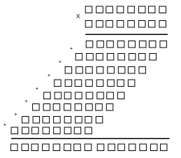 |  |
But not everything is as smooth as we would like. Unlike the positional number system, the following operations (called "non-modular") are more complicated than in the positional number system: comparing numbers, overflow control, division, square root, etc. The first successful attempts to use modular arithmetic in microelectronics were made back in the 1950s, but due to difficulties with non-modular operations, interest was somewhat abated. However, at present modular arithmetic is again returning to microelectronics for the following reasons:
- widespread use of mobile processors that require high speed with low power consumption. The lack of transfer in the arithmetic operations of addition / multiplication can reduce energy consumption.
- the increasing density of elements on the chip in some cases does not allow for full testing; therefore, the importance of the stability of processors to possible errors is growing.
- the emergence of specialized processors with a large number of operations on vectors that require high speed and include mainly the addition and multiplication of numbers (as an example, matrix multiplication, scalar product of vectors, Fourier transforms, etc.).
Currently, modular arithmetic is used in the following areas: digital signal processing, cryptography, image processing / audio / video, etc.
Direct conversion
A direct conversion from a positional number system (usually in binary form) to a number system in residuals consists in finding the remainder of division for each of the modules of the system.
Example : Suppose you want to find a representation of the number X = 25 from a system of modules (3, 5, 7). X = (25% 3, 25% 5, 25% 7) = (1, 0, 4).
The implementation of finding the residue in microelectronics for a given module is based on the following properties of the residues:
(a + b)% p = (a% p + b% p)% p
(a * b)% p = (a% p * b% p) % p
Any number X can be written as X% p = (x n-1 * 2 n-1 + x n-2 * 2 n-2 + x 0 * 2 0 )% p = ((x n-1 ) % p * 2 n-1 % p) + ((x n-2 )% p * 2 n-2 % p) + ... + x 0 % p)% p. Since in this case x n-1 , ... x 0 are 0 or 1, in fact, we need to add the residues of the form (2 i % p).
Example : let the number 25 be given or in the binary number system 11001 and you want to find the remainder modulo 7.
25% 7 = (1 * 2 4 + 1 * 2 3 + 0 * 2 2 + 0 * 1 + 1 * 2 0 )% 7 = (2 4 % 7 + 2 3 % 7 + 1% 7)% 7 = (2 + 1 + 1)% 7 = 4
The system of modules used is selected for a specific task. For example, to represent 32-bit numbers, the following system of modules is enough: (7, 11, 13, 17, 19, 23, 29, 31) - they are all mutually simple with each other, their product is 6685349671> 4294967296. Each of the modules is not exceeds 5 bits, that is, operations of addition and multiplication will be performed on 5-bit numbers.
Of particular importance is the system of modules of the form: (2 n -1, 2 n , 2 n +1) due to the fact that the direct and inverse transformations for them are performed in the simplest way. To get the remainder of dividing by 2 n, it is enough to take the last n digits of the binary representation of the number.
Arithmetic operations
Example : let a system of modules (3, 5, 7) be given, that is, we can perform operations whose result does not exceed 3 * 5 * 7 = 105. We multiply two numbers 8 and 10.
8 = (8% 3, 8% 5 , 8% 7) = (2, 3, 1)
10 = (10% 3, 10% 5, 10% 7) = (1, 0, 3)
8 * 10 = ((2 * 1)% 3, ( 3 * 0)% 5, (1 * 3)% 7) = (2, 0, 3)
Check
80 = (80% 3, 80% 5, 80% 7) = (2, 0, 3)
Inverse transformation
The inverse transformation from the number system in residual classes to the positional number system is performed in one of two ways:
- Based on the Chinese remainder theorem or a system of orthogonal bases
- Based on a polyadic code (other names mixed-radix system, mixed base system)
The rest of the methods proposed in various literature, in fact, are a mixture of these two.
A method based on the Chinese remainder theorem is based on the following idea:
X = (x 1 , x 2 , ... x n ) = (x 1 , 0, ..., 0) + (0, x 2 , ..., 0) + ... + (0, 0, ..., x n ) = x 1 * (1, 0, ..., 0) + x 2 * (0, 1, ..., 0) + ... + x n * (0, 0, …, 1).
That is, for the inverse transformation, it is required to find a system of orthogonal bases B1 = (1, 0, ..., 0), B2 = (0, 1, ..., 0), ..., BN = (0, 0, ..., 1). These vectors are found once for a given basis, and for their search it is necessary to solve an equation of the form: (M i* b i )% p i = 1, where M i = M / p i , and b i is the desired number. In this case, the positional representation B i = M i * b i and
X = (x 1 * (M 1 * b 1 ) + x 2 * (M 2 * b 2 ) + ... + x n * (M n * b n ))% M
Example : Let a system of modules be given (3, 5, 7), we will find the values of M i and b i (0 <i <= 3)
M = 3 * 5 * 7 = 105
M 1 = 105/3 = 35
M 2 = 105 / 5 = 21
M 3 = 105/7 = 15
(35 * b 1 )% 3 = 1 => b 1 = 2
(21 * b 2 )% 5 = 1 => b 2 = 1
(15 * b 3 ) % 7 = 1 => b 3 = 1
Now we transform some number in the system of residual classes. Put
X = (2, 3, 1) = (2 * 35 * 2 + 3 * 21 * 1 + 1 * 15 * 1)% 105 = (140 + 63 + 15)% 105 = 218% 105 = 8
The disadvantage of this method is that the inverse transformation requires the multiplication and addition of large numbers (M 1 , ..., M n ), as well as the operation of taking the remainder modulo a large number M.
A method based on a polyadic code is based on the idea that any number X can be represented in a system of coprime numbers p 1 , ... p n , as [4]:
X = a 1 + a 2 * p 1 + a 3 * p 1 * p 2 + ... + a n-1 * p 1 * p 2 * ... * p n-2 + a n * p 1 * p2 * ... * p n-1 , where 0 <a i <p i
- X% p 1 = x 1 = a 1
- (X - a 1 )% p 2 = (x 2 - a 1 )% p 2 = (a 2 * p 1 )% p 2 => a 2 = ((p 1 -1 )% p 2 * (x 2 - a 1 ))% p 2
- (X - a 1 - a 2 * p 1 )% p 3 = (a 3 * p 1 * p 2 )% p 3 => a 3 = ((p 2 -1 )% p 3 * ((p 1 - 1 )% p 3 * (x 3 - a 1 ) - a 2 ))% p 3
- ...
To use this method, constants of the form (p i -1 )% p k -1 are required . You can also notice that it is possible to start the calculation of a 3 as soon as the value of a 1 appears . Conveyor converters can be built on the basis of this method.
Example : Consider the same example - find the positional representation of the number X = (2, 3, 1) in the module system (3, 5, 7)
- a 1 = x 1 = 2
- a 2 = ((p 1 -1 )% p 2 * (x 2 - a 1 ))% p 2 = ((3 -1 )% 5 * (3 - 2))% 5 = 2 * 1 = 2
- a 3 = ((p 2 -1 )% p 3 * ((p 1 -1 )% p 3 * (x 3 - a 1 ) - a 2 ))% p 3 = ((5 -1 )% 7 * ((3 -1 )% 7 * (1 - 2) - 2))% 7 = (3 * (5 * (1-2) -2))% 7 = (3 * (- 7))% 7 = 0
- X = a 1 + a 2 * p 1 + a 3 * p 1 * p 2 = a 1 + 3 * a 2 + 15 * a 3 = 2 + 3 * 2 + 15 * 0 = 8
Note : in order to find a constant of the form (3 -1 )% 5, it is necessary to solve the equation (3 * x)% 5 = 1, where 0 <= x <5
PS
The article was written somewhat messy, because the topic is large enough and it is not possible to fit everything into one article. In the following articles I will try to describe in more detail the various aspects of modular arithmetic. On Habr, I did not find anything at all that relates to this topic, only brief references in other articles, so it was decided to write a short review with simple examples. For those who are interested in the topic, I recommend reading book number [3] from the list of references (in English), it is written in an accessible language with a large number of examples.
Literature
[1] en.wikipedia.org/wiki/%D0%9F%D0%BE%D0%B7%D0%B8%D1%86%D0%B8%D0%BE%D0%BD%D0%BD%D0% B0% D1% 8F_% D1% 81% D0% B8% D1% 81% D1% 82% D0% B5% D0% BC% D0% B0_% D1% 81% D1% 87% D0% B8% D1% 81% D0% BB% D0% B5% D0% BD% D0% B8% D1% 8F
[2] en.wikipedia.org/wiki/%D0%9A%D0%B8%D1%82%D0%B0%D0%B9 % D1% 81% D0% BA% D0% B0% D1% 8F_% D1% 82% D0% B5% D0% BE% D1% 80% D0% B5% D0% BC% D0% B0_% D0% BE% D0 % B1_% D0% BE% D1% 81% D1% 82% D0% B0% D1% 82% D0% BA% D0% B0% D1% 85
[3] Amos Omondi, Benjamin Premkumar, Residue Number Systems: Theory and Implementation , 2007.
[4] MA Soderstrand, WK Jenkins, GA Jullien and FJ Taylor. 1986. Residue Number System Arithmetic: Modern Applications in Digital Signal Processing, IEEE Press, New York.