Quickly compute accurate 3D distance maps using CUDA technology

The Distance Map is an object that allows you to quickly get the distance from a given point to a specific surface. Usually a matrix of distance values ​​for nodes with a fixed pitch. It is often used in games to determine “getting” into a player or object, and for optimization tasks in combining objects: position objects as close to each other as possible, but so that they do not overlap. In the first case, the quality of the distance map (that is, the accuracy of the values ​​in the nodes) does not play a big role. In the second, life can depend on it (in a number of applications related to neurosurgery). In this article I will tell you how to accurately calculate the distance map in a reasonable time.

Main objects

Suppose we have some surface S defined by a set of voxels. The voxel coordinates will be counted on a regular grid (i.e. the steps along X, Y and Z are the same).

It is required to calculate the distance map M [X, Y, Z] for all voxels that lie in the cube containing the surface; M [x, y, z] = d ((x, y, z), S) = min (d ((x, y, z), (S _n x, S _n y, S _n z)) = sqrt (min ((xS _n x) ² + (yS _n y) ² + (zS _n z) ² )). The last equality is true only for a regular grid, the rest should be obvious.

Where does the data come from

For our task, the data comes from an MRI device . Let me remind you that we work with 3D images, so the entire 3D image is a set of flat images for different slices in Z, which I certainly can not imagine here; they are slightly smaller than the X and Y resolution. Typical tomography size is about 625x625x592 voxels.


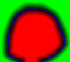
As a result of rather tricky transformations, the border of the surface of the head stands out. The very essence of these transformations comes down to a variety of filters that remove the “noise” and the function that determines the boundary itself by the gradient. There is nothing new here; similar things were discussed in the subject of “Image Processing”, in particular . The border itself is the target set to which we will calculate distances and build a map.

Direct search

First, let’s figure out why not fill the distance map with “by definition” values ​​- minimums of distances to border points. Total points of the map: X * Y * Z, surface points of the order of max (X, Y, Z) ² . Recall the sizes of the source data and get something of the order of 592 * 625 ⁴ arithmetic-logical operations. The calculator will tell you that it is more than 90,000 billion. To put it mildly, a bit too much, we will postpone for now a direct search.

Dynamic programming

It begs the use of the fact that data is represented in a three-dimensional array; you can somehow calculate the value at each point using its neighbors, and of course we are not the first to do this. The fact that keeping a structure of 592 * 625 * 625 * sizeof (float) in size, which is about 1 Gigabyte, is somewhat resource-intensive, is somewhat repulsive. Well, ok, let’s forget so far that tomography can be shot with double resolution (another 8 times more) - 640Kbytes has long been lacking.

The most trivial method of filling (city-block), similar to the algorithm for bypassing the labyrinth , fulfills in a matter of seconds, but the maximum error on a three-dimensional grid can be 42 grid steps for the maximum calculated distance of 50 steps. How bad is that? Complete failure.

The only algorithm from the class ( central point ) gives an almost satisfactory accuracy (error of no more than 0.7 grid steps), but minutes work.

We tried to find a compromise by implementing the chessboard distance (the description is in the same article as the central point), but the final accuracy could not be arranged, and its operation time was tens of seconds.

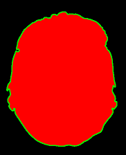
The picture is a link to a full-sized one, but even the preview shows “strange” behavior far enough from surface points, and especially if you also need to calculate internal objects. On the left is the chessboard, and on the right is what was obtained by direct enumeration. And once again I remind you, for those who look only at pictures - we are talking about 3D images, so the strange "punctures" inside are understandable - they are caused by proximity to the surface on the next or previous Z slides. In general, a failure.

Direct search again

Yes, the word CUDA in the picture is hinting. Maybe 90,000 billion - not so much, or maybe this number can be somehow reduced, without loss of accuracy. In any case, the middle-end video card handles primitive computing operations 80-120 times faster than a processor of the same class. Let's try it.

Yes, and direct enumeration has a significant advantage - there is no need to keep the entire distance map in memory, and as a result - linear scalability.

Bust Reduction

Thesis: it makes no sense for each point to check the distance to each point of the border. In fact, the distance map is required to provide good accuracy only in close proximity to the border, rather distant points can not be considered at all, and intermediate points should be marked with an approximate distance.

The correctness criterion is absolute accuracy near the border (at a distance of up to 10 (GUARANTEED_DIST) grid steps), good accuracy at a distance of 36 (TARGET_MAX_DIST) steps, and visual adequacy (without artifacts - why confuse surgeons). The numbers 10 and 36 are taken directly from our task (we generally have these values ​​in millimeters and the millimeter grid).

Cubic index

For each point, I would like to determine how accurately its value needs to be calculated. Obviously, the size of such a structure will coincide with the size of the original image, and this is a lot, and will be considered for a long time.

We will merge the points into “cubes”. Let the cube size be 32 (CUBE_SIZE), then the index will have dimensions 20 x 20 x 19. We

mark the cube according to the type of “best” point lying in it. If at least one point requires accurate calculation, we consider the entire cube for sure. In the worst case, we do not consider it at all.

How to quickly label cubes? Let's start from the border points: add to each of them the offset GUARANTEED_DIST in all 27 directions ((-1,0,1) x (-1,0,1) x (-1,0,1)), we get the index of the corresponding cube, dividing by 32 (CUBE_SIZE), and mark it as “exact” - after all, it contains at least one point that requires accurate calculation. Task: to explain why this is enough, and all the cubes containing points for accurate calculation will be marked correctly.

Just in case, the pretty trivial code that executes this is:

  for (size_t t = 0; t < borderLength; t++)
  {
    for (int dz = -1; dz <= 1; dz++)
      for (int dy = -1; dy <= 1; dy++)
        for (int dx = -1; dx <= 1; dx++)
        {
          float x = border[t].X + (float)dx * GUARANTEED_DIST;
          float y = border[t].Y + (float)dy * GUARANTEED_DIST;
          float z = border[t].Z + (float)dz * GUARANTEED_DIST;
          if (x >= 0 && y >= 0 && z >= 0)
          {
            size_t px = round(x / CUBE_SIZE);
            size_t py = round(y / CUBE_SIZE);
            size_t pz = round(z / CUBE_SIZE);
            size_t idx = px + dim_X * (py + skip_Y * pz);
            if (idx < dim_X * dim_Y * dim_Z)
            {
              markedIdx[idx] = true;
            }
          }
        }
  }


Based on practical data, this idea made it possible to reduce the order of enumeration of “everything” by 4-5 times. All the same, it turns out a lot, but the idea with cubes is still useful to us.

Cubic container

In fact, it makes no sense to calculate the distance to all points of the boundary; it is enough to calculate it only for the nearest points; and now we know how to organize such a structure.

We will scatter all voxels of border S into cubes (we will forget about index cubes from now on; we built them, understood how to use them, and now we don’t work with them anymore). In each cube we will put those border points that are reachable (lie at a distance of TARGET_MAX_DIST and less). To do this, just calculate the center of the cube, and put aside the distance sqrt (3) / 2 * CUBE_SIZE (this is the diagonal of the cube) + TARGET_MAX_DIST. If the point is reachable from the top of the cube or any point on the side, then it is reachable from its inside.

I think it makes no sense to give the code, it is very similar to the previous one. And the correctness of the idea is also obvious, but one essential point remains: in fact, we “multiply” the border points, the number of which can increase up to 27 times with a reasonable TARGET_MAX_DIST (smaller than the cube size) and even more times differently.

Optimization:

• The first (forced) - the size of the cube is selected so that the total number of "multiplied" points is not more than the maximum amount of memory on them (we took 512 megabytes). You can choose the cube size quickly (a little math).
• The second (reasonable) is to use indices for the initial and final placement of points for each cube, these indices can intersect, and due to their competent calculation, you can save another 2 times in memory size.

I will not consciously give exact algorithms for both points (what if you implement them better and become our competitors?;)), There are more words than ideas.

In general, the cubes reduce the search order by X / CUBE_SIZE * Y / CUBE_SIZE * Z / CUBE_SIZE times, but we must remember that reducing the size of the cube will require significantly more memory, and the threshold value for our images turned out to be around 24-32.

Thus, the task was reduced to about 100-200 billion material operations. Theoretically, this is computable on a graphics card in tens of seconds.

CUDA Kernel

It turned out so simple and beautiful that I’m not too lazy to show it:

__global__ void minimumDistanceCUDA( /*out*/ float *result,
                   /*in*/ float *work_points,
                   /*in*/ int  *work_indexes,
                   /*in*/ float *new_border)
{        
  __shared__ float sMins[MAX_THREADS]; // max threads count
  
  for (int i = blockIdx.x; i < BLOCK_SIZE_DIST; i += gridDim.x)
  {
    sMins[threadIdx.x] = TARGET_MAX_DIST*TARGET_MAX_DIST;

    int startIdx = work_indexes[2*i];
    int endIdx  = work_indexes[2*i+1];    
    
    float x = work_points[3*i];
    float y = work_points[3*i+1];
    float z = work_points[3*i+2];
    
    // main computational entry
    for (int j = startIdx + threadIdx.x; j < endIdx; j += blockDim.x)
    {        
      float dist = (x - new_border[3*j] )*(x - new_border[3*j] )
            + (y - new_border[3*j+1])*(y - new_border[3*j+1])
            + (z - new_border[3*j+2])*(z - new_border[3*j+2]);
      if (dist < sMins[threadIdx.x])
        sMins[threadIdx.x] = dist;
    }

    __syncthreads();

    if (threadIdx.x == 0)
    {
      float min = sMins[0];      
      for (int j = 1; j < blockDim.x; j++)
      {
        if (sMins[j] < min)
          min = sMins[j];
      }
      result[i] = sqrt(min);
    }        

    __syncthreads();
  }
}


We load the coordinate block of the distance map points for enumeration (work_points), the corresponding start and end indices for enumeration of border points (work_indexes), and the border optimized by the algorithm with cubes (new_border). We take the results in single material accuracy.

Actually, the kernel code itself, which is very nice to understand, even without the intricacies of CUDA. Its main feature is the use of the gridDim.x and threadIdx.x variables denoting the indices of the current thread from the set of running threads on the video card - everyone does the same thing, but with different points, and then the results are synchronized and accurately recorded.

It remains only to correctly organize the calculation of work_points on the CPU (but it's so easy!) And start the calculator:

#define GRID       512   // calculation grid size
#define THREADS     96   // <= MAX_THREADS, optimal for this task
minimumDistanceCUDA<<>>(dist_result_cuda, work_points_cuda, work_indexes_cuda, new_border_cuda);


On a Core Duo E8400 and a GTX460 graphics card, average tomography is processed within a minute , the memory consumption is limited to 512MB. The distribution of processor time is approximately 20 percent on the CPU and file operations, and the remaining 80 on the calculation of the lows on the video card.

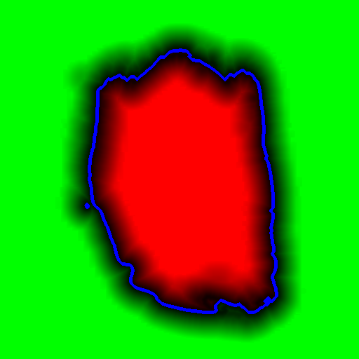
And here is the picture counted with the “roughening” of distant points:



Somehow, I hope something comes in handy. A big request, do not copy pictures and do not re-publish without my permission (I am the author of the method, although it is difficult to call it a "method").

Have a good day!