History of Electronic Computers, Part 3: ENIAC
- Transfer
Other articles of the cycle:
- Relay history
- История электронных компьютеров
- История транзистора
The second project to create an electronic computer that emerged as a result of the war, like the Colossus, required a lot of minds and hands for a fruitful realization. But, like the Colossus, he would never have appeared if he hadn’t been a single person obsessed with electronics. In this case, his name was John Mouchli .
Mauchly's story is intertwined in mysterious and suspicious ways with the story of John Atanasoff. As you remember, we left Atanasov and his assistant Claude Berry in 1942. They gave up work on the electronic computer and started other military projects. Mouchly had a lot in common with Atanasov: both of them were professors of physics in little-known institutions that did not possess prestige and authority in wide academic circles. Mauchly languished in isolation as a teacher at the tiny Ursinus College on the outskirts of Philadelphia, who did not even have such a modest prestige as that of the state of Iowa, where Atanasov worked. None of them did anything to attract the attention of their more elite counterparts from, say, the University of Chicago. However, both captured eccentric idea: to build a computer from electronic components,
John mochly
Predicting the weather
For a while these two men established a definite connection. They met in the late 1940s at the conference of the American Association for the Advancement Science (AAAS) in Philadelphia. There, Mouchli gave a presentation on his study of cyclical patterns in weather data using the electronic harmonic analyzer he developed himself. It was an analog computer (that is, it represented values not in digital form, but in the form of physical quantities, in this case, current — the greater the current, the greater the value), similar in work with the mechanical tide predictor developed by William Thomson (later Lord Kelvin) in the 1870s.
Atanasov, who was sitting in the hall, knew that he had found a comrade on a lonely journey into the country of electronic computing, and without delay, went to Mouchli after his report to tell him about the car he had built in Ames. But to understand how, in general, Mouchli found himself on the scene with his presentation of an electronic weather computer, it was necessary to return to his roots.
Mouchley was born in 1907 in the family of physicist Sebastian Mouchli. Like many of his contemporaries, he became interested in radio and electronic lamps as a boy, and hesitated between the careers of an electronics engineer and a physicist before deciding to concentrate on meteorology at Johns Hopkins University. Unfortunately, after graduation, he fell right into the clutches of the Great Depression, and was grateful for getting a job in Ursinus in 1934 as the only member of the Faculty of Physics.
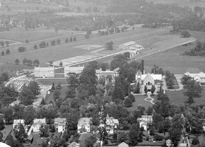
Ursinus College in 1930
In Ursinus, he took up the dream project - unraveling the hidden cycles of the global natural machine, and learning how to predict the weather not for days, but for months and years ahead. He was convinced that the Sun controls the weather patterns, which last for several years, related to solar activity and spots. He wanted to extract these patterns from the huge amount of data accumulated by the US Meteorological Bureau with the help of students and a set of desktop calculators purchased for pennies from failed banks.
It soon became clear that there was too much data. Machines could not carry out calculations quickly enough, and in addition human errors began to manifest themselves with constant copying of the intermediate results of the machine onto paper. Mouchly began to think about a different way. He knew about electron-tube counters first created by Charles Wynn-Williams, which his fellow physicists used to count subatomic particles. Considering that electronic devices obviously could record and accumulate numbers, Mouchly became interested, why shouldn't they perform more complex calculations? For several years in his spare time, he played with electronic components: switches, counters, substitution cipher machines, using a mixture of electronic and mechanical components, and a harmonic analyzer, he used for a weather prediction project, retrieving data similar to multi-week patterns of precipitation fluctuations. It was this discovery that led Mouchli to AAAS in 1940, and then Atanasov to Mouchli.
Visit
The key event of the relationship between Mouchli and Atanasov occurred six months later, in the early summer of 1941. In Philadelphia, Atanasov told Mouchli about the electronic computer he had built in Iowa, and mentioned how cheap it had cost him. In their subsequent correspondence, he continued to make intriguing hints about how he built his computer at a cost of no more than $ 2 per rank. Mouchli became interested and was very surprised by this achievement. By that time, he was already carrying serious plans to build an electronic calculator, but without the support of the college he would have to pay for all the equipment from his pocket. For one lamp, they usually asked for $ 4, and at least two lamps were required to store one binary digit. How, he thought, did Atanasov manage to save so well?
After six months, he finally had time to go west to satisfy his curiosity. After one and a half thousand kilometers in a car, in June 1941, Mouchley and his son came to visit Atanasov in Ames. Mouchli later told me that he had left disappointed. Atanasov’s cheap data storage was not at all electronic, but held by electrostatic charges on a mechanical drum. Because of this, and because of other mechanical parts, as we have already seen, he could not perform calculations at speeds even approaching those that Mouchley dreamed of. Later he called it "a mechanical knickknack using several electron tubes." However, shortly after the visit, he wrote a letter praising Atanasov’s car, where he wrote that it was “essentially electronic, and solved in just a few minutes any system of linear equations, included no more than thirty variables. " He argued that it could be faster and cheaper than mechanicalBush's differential analyzer .
Thirty years later, the relationship between Mouchli and Atanasov will be key in the Honeywell vs Sperry Rand litigation, as a result of which the applications for patents for the electronic computer created by Mouchli were revoked. Without saying anything about the merit of the patent itself, despite the fact that Atanasov was a more experienced engineer, and given Mouchli’s suspicious opinion about Atanasoff’s computer, expressed in hindsight, there is no reason to suspect that Mouchli learned or copied something important from Atanasov’s work. But more importantly, the ENIAC scheme has nothing to do with the Atanasoff-Berry computer. The maximum that can be said is that Atanasov spurred Mauchly’s confidence, proving the possibility that the electronic computer could work.
School of Moore and Aberdeen
And at this time Mouchli was in the same place from which he started. There was no magic focus for cheap electronic storage, and while he remained in Ursinus, he did not have the means to make the electronic dream come true. And then he was lucky. In the summer of 1941, he studied in the summer course in electronics at the Moore School of Engineering at the University of Pennsylvania. By that time France was already occupied, Britain was under siege, submarines plied the Atlantic, and America’s relations with aggressive expansionist Japan were deteriorating rapidly [and Hitler Germany attacked the USSR / approx. trans.]. Despite the isolationist sentiment among the population, American intervention seemed possible, and probably unavoidable, to elite groups from places like the University of Pennsylvania.
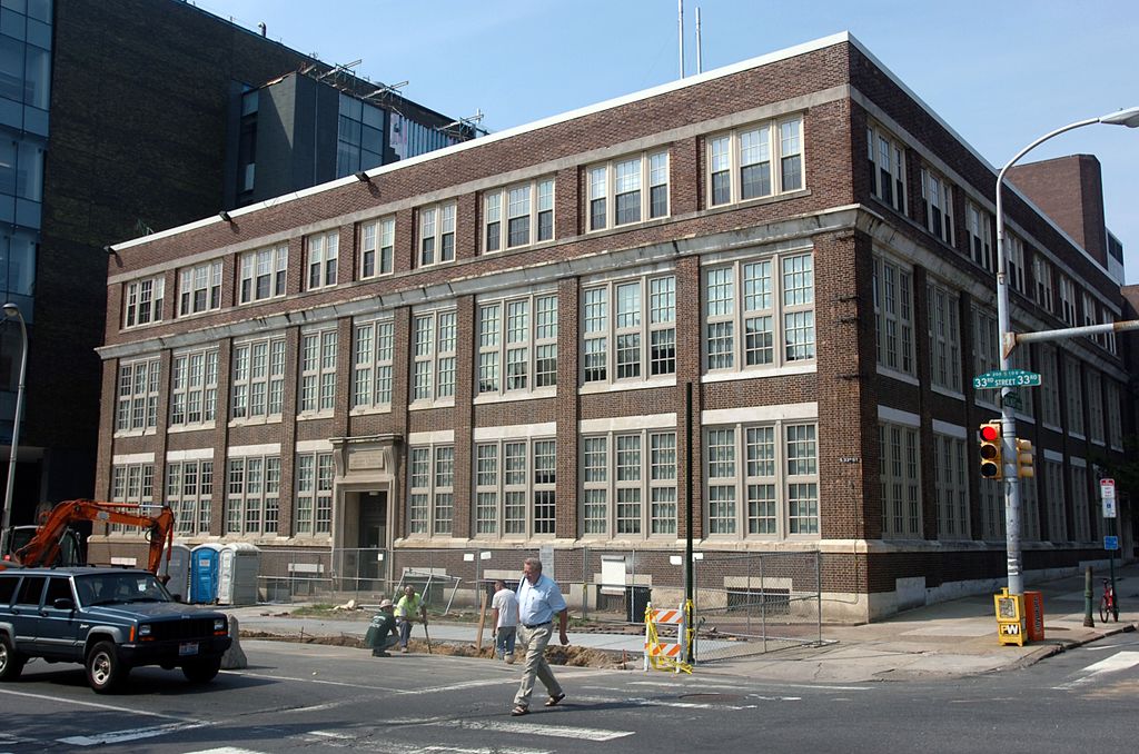
Moore’s School of Engineering
led to two major consequences for Mouchley: first, he tied him to John Presper Eckert, nicknamed Pres, from a local family of real estate magnates, and a young wizard of electronics who spent his days in the laboratory of television pioneer Phil Farnsworth . Later, Eckert will share the patent (which is then invalidated) on ENIAC from Mouchley. Second, it provided Mouchley a place at the Moore School, ending his long academic isolation in the swamp of Ursinus College. This, apparently, was not due to any special merits of Mouchli, but simply because the school desperately needed people to be replaced by scientists who had left to work on military orders.
But by 1942, most of the school of Mura herself began working on a military project: counting ballistic trajectories with the help of mechanical and manual work. This project grew out of the existing connection between the school and the Aberdeen testing ground, located 130 km further along the coast, in Maryland.
The landfill was created during World War I to test artillery, to replace the previous landfill in Sandy Hook, New Jersey. In addition to direct shooting, his task was to count fire tables used by artillery in combat. Air resistance did not allow to calculate the projectile landing site, simply by solving a quadratic equation. Nevertheless, high accuracy was extremely important for artillery fire, since it was the first shots that ended with the greatest defeat of the enemy forces - after them the enemy quickly hid under the ground.
To achieve this accuracy, modern armies made up detailed tables that told the shooters how far their projectile would land after being shot at a certain angle. The compilers used the initial speed and location of the projectile to calculate its location and speed over a short time interval, and then repeated the same calculations for the next interval, and so on, hundreds and thousands of times. For each combination of gun and projectile such calculations needed to be carried out for all possible firing angles, taking into account different atmospheric conditions. The counting load was so large that in Aberdeen the calculations of all tables, begun at the end of the First World War, were completed only by 1936.
Obviously, Aberdeen needed a better solution. In 1933, he concluded an agreement with Moore’s school: the army will pay for the construction of two differential analyzers, analog computers created according to the MIT scheme under the direction of Vanévar Bush . One will be sent to Aberdeen, and the other will remain at the disposal of Moore’s school and will be used at the discretion of the professorate. The analyzer could build a trajectory in fifteen minutes, which would take a person several days to calculate, although the accuracy of computer calculations was slightly lower.
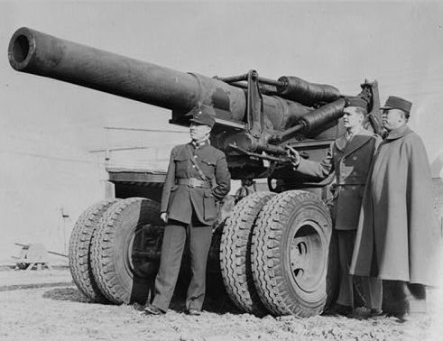
Demonstration howitzers in Aberdeen, approx. 1942
However, in 1940, the research unit, now called the Ballistic Research Laboratory (Ballistic Research Laboratory, BRL), requested its car, which was at Moore’s school, and began calculating artillery tables for the impending war. The counting group of the school was also attracted to support the machine with the help of people-calculators. By 1942, 100 women calculators in the school worked six days a week, grinding up calculations for the war — among them was Mouchley's wife, Mary, who worked on the firing tables of Aberdeen. Mouchly was made head of another computer team working on calculations for radar antennas.
From the day he arrived at Moore’s school, Mouchly promoted his idea of an electronic computer throughout the department. He already had significant support in the person of Presper Eckert andJohn Brainerd , a senior faculty member. Mouchley provided the idea, Eckert provided the engineering approach, and Brainerd provided persuasiveness and legitimacy. In the spring of 1943, this troika decided that the time had come to advertise Mauchly’s long-standing idea to the army. But the mysteries of the climate, which he had long tried to solve, had to wait. The new computer was supposed to serve the needs of the new host: to track not the eternal sinusoids of global temperature cycles, but the ballistic trajectories of artillery shells.
ENIAC
In April 1943, Mouchley, Eckert, and Brainerd drafted the “Electronic Differential Analyzer Report”. This brought into their ranks another ally, Hermann Goldstein , a mathematician and army officer who served as a mediator between Aberdeen and the school of Moore. With the help of Goldstein, the group presented the idea to the BRL committee, and received a military grant, with Brainerd as the project's scientific adviser. They needed to complete the creation of the machine by September 1944 with a budget of $ 150,000. The team called the project ENIAC: Electronic Numerical Integrator, Analyzer and Computer (Electronic Numerical Integrator and Computer).
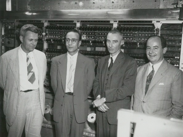
From left to right: Julian Bigelow, Herman Goldstein, Robert Oppenheimer, John von Newman. Picture taken at the Princeton Institute of Advanced Studies after the war, with a later computer model
As in the case of the Colossus in Britain, authoritative engineering authorities in the United States, for example, the National Defense Research Committee (NDRC), were skeptical of the ENIAC project. Moore’s school did not have the reputation of an elite educational institution, but it offered to create something unheard of. Even industrial giants such as RCA hardly managed to create relatively simple electronic counter circuits, not to mention a customizable electronic computer. George Stibits, the architect of the relay computers at Bell's lab, who was then working on the NDRC project, believed that it would take too long to create ENIAC to be useful in the war.
In this he was right. The creation of ENIAC will take twice as much time and three times more funds than originally planned. He sucked the solid part of the human resources of Moore’s school. For development alone, seven more people needed to be involved, in addition to the initial group of Mouchley, Eckert and Brainerd. Like the Colossus, ENIAC attracted many people-calculators to help set up their electronic replacement. Among them were the wife of Hermann Goldstein Adele, and Gene Jennings (later Bartik), who later had an important job of developing computers. The NI letters in the ENIAC title suggested that the Moore school provided the army with a digital, electronic version of a differential analyzer that would solve the integrals for the trajectories faster and more accurately than its analog mechanical predecessor.
Part of the project’s ideas could have been borrowed from the 1940 proposal made by Irven Travis. It was Travis who participated in the signing of the contract for Moore’s use of the analyzer in 1933, and in 1940 he proposed an improved version of the analyzer, although not electronic, but working on a digital principle. He had to use mechanical meters instead of analog wheels. By 1943, he had left Moore’s school and occupied the post in the leadership of the fleet in Washington.
The basis of ENIAC capabilities, again, like the Colossus, was a variety of functional modules. The most commonly used batteries for addition and calculation. Their scheme was taken from the Winn-Williams electronic meters used by physicists, and they literally did the addition with the help of an account, as the preschoolers think on fingers. Other functional modules included multipliers, function generators that searched for data in tables, which replaced the calculation of more complex functions like sine and cosine. Each module had its own software settings, with the help of which a small sequence of operations was set. Like the Colossus, programming was carried out using a combination of a panel with switches and similar to telephone switches panel with sockets.
ENIAC had several electromechanical parts, in particular, a relay register that served as a buffer between electronic batteries and IBM punch machines used for input and output. This architecture was very similar to the Colossus. Sam Williams from Bell Laboratories, who collaborated with George Stibitz on Bella relay computers, also built a register for ENIAC.
The key difference from the Colossus made ENIAC a more flexible machine: the ability to program the main settings. The main programmable device sent pulses to functional modules that caused the launch of pre-installed sequences, and received response pulses upon completion of work. Then it passed to the next operation in the main control sequence, and produced the necessary calculations as a function of a set of smaller sequences. The main programmable device could make decisions using a stepper motor: a ring counter, which determined which of the six output lines to redirect the impulse to. In this way, the device could perform up to six different functional sequences, depending on the current state of the stepper motor. This flexibility will allow ENIAC to solve problems
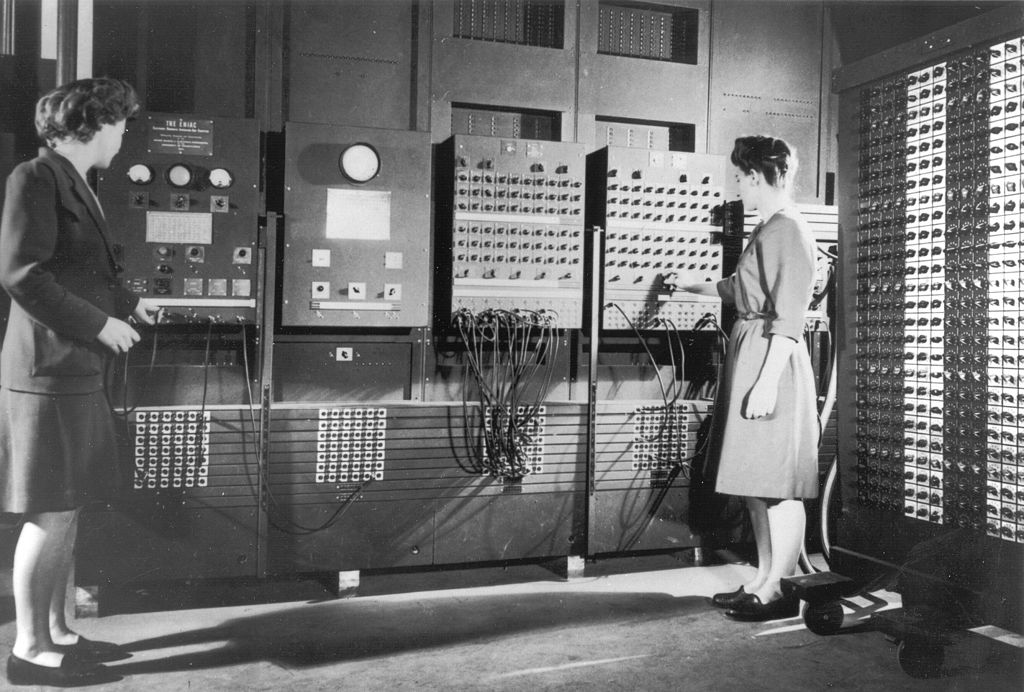
Configure ENIAC using switches and switches
Eckert was responsible for ensuring that all the electronics in this monster buzzed and buzzed, and he himself came up with the same basic tricks as Flowers in Bletchley: the lamps must operate at currents much smaller than the standard ones and the car does not have to be turned off. But because of the huge number of lamps used, one more trick was needed: plug-ins, each of which had several dozens of lamps mounted, could be easily removed and replaced if they failed. Then, without haste, the maintenance staff found and replaced the failed lamp, and ENIAC was immediately ready for operation. And even with all these precautions, given the huge number of lamps in ENIAC, he could not do task calculations all weekend or all night, as relay computers did. At some point, the lamp must have blown.
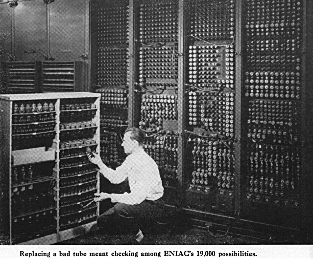
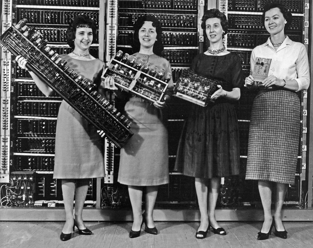
An example of a variety of lamps in ENIAC. ENIAC
reviews often mention its enormous size. Rows of racks with lamps — there were 18,000 of them in all — switches and switches would have occupied a typical country house and lawn in front of it to boot. Its size was due not only to its components (the lamps were relatively large), but also to a strange architecture. And although all computers of the mid-century seem to be large in terms of modern concepts, the next generation of electronic computers was much smaller than ENIAC, and had great potential when using one-tenth of electronic components.
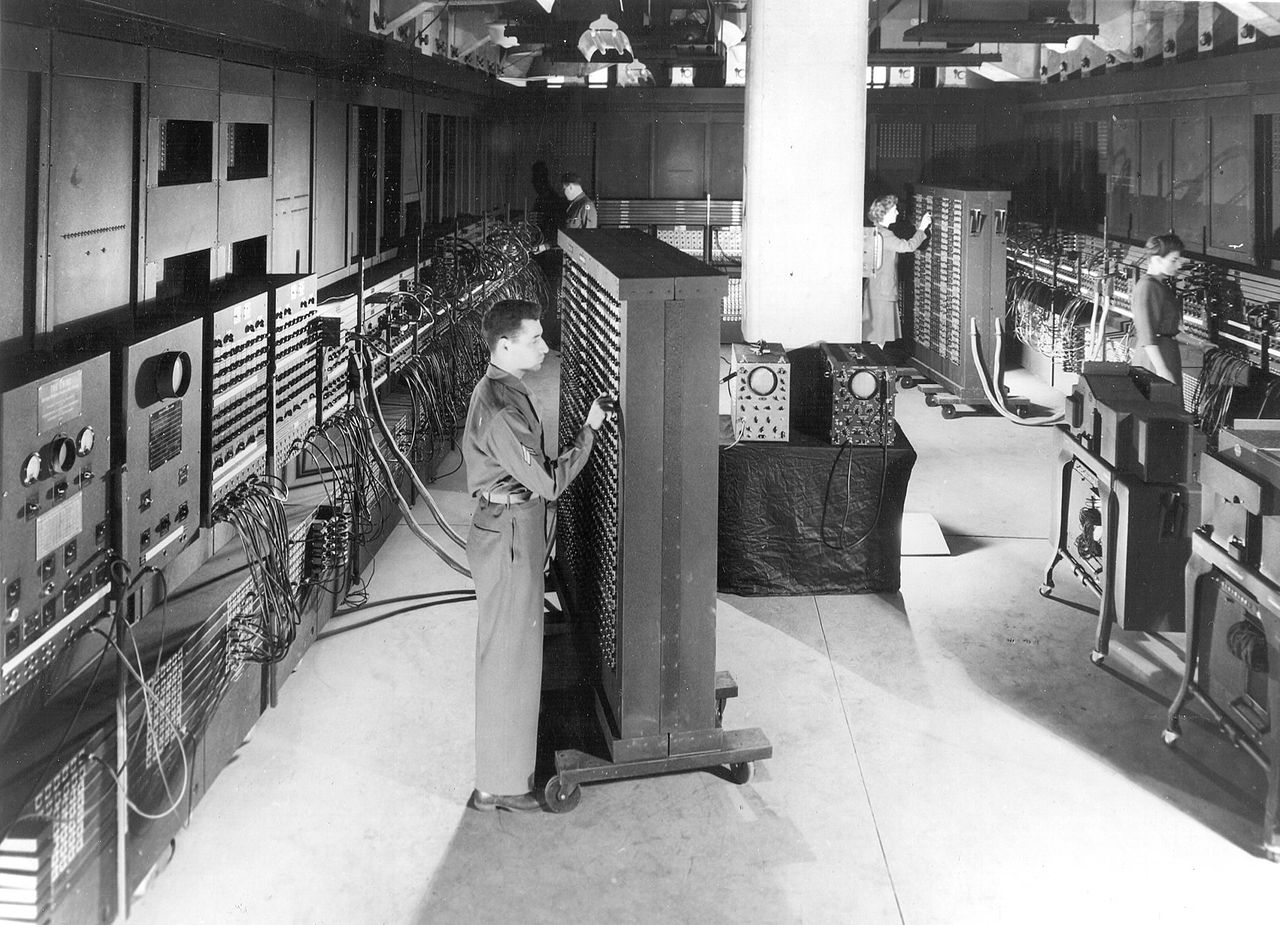
ENIAC Panorama at Moore’s School
The grotesque size of ENIAC stems from two main design solutions. The first sought to increase the potential speed at the expense of cost and complexity. After that, almost all computers stored numbers in registers, and processed them in separate arithmetic modules, again storing the results in the register. ENIAC did not separate storage and processing modules. Each number storage module was at the same time a processing module capable of adding and subtracting, which required much more lamps. It could be considered as a strongly accelerated version of the Moore's calculator department at Moore’s school, since “its computational architecture resembled twenty calculator people working with ten-digit desktop calculators that transmit the results of the calculations to and fro.”
The second design decision is more difficult to justify. Unlike ABC or Bell relay machines, ENIAC did not store numbers in binary. He translated decimal mechanical calculations directly into electronic form, with ten triggers for each digit — if the first burned, it was zero, the second 1, the third 2, and so on. It was a huge expense of expensive electronic components (for example, to represent the number 1000 in binary form requires 10 triggers, one per binary digit (1111101000); and in the ENIAC scheme this required 40 triggers, ten per decimal digit), which apparently, it was organized only because of the fear of possible transformation difficulties between the binary and decimal systems. However, the Atanasoff-Berry computer, the Colossus, and the relay machines Bella and Zuse used the binary system,
No one will repeat such design decisions. In this sense, ENIAC was similar to ABC - a unique wonder, not a template for all modern computers. However, his advantage was that he proved, beyond any doubt, the performance of electronic computers, performing useful work, and solving real problems with surprising speed for others.
Rehabilitation
By November 1945, ENIAC was fully operational. He could not boast the same reliability as his electromechanical relatives, but he was reliable enough to use his speed advantage several hundred times. The calculation of the ballistic trajectory, which took fifteen minutes for a differential analyzer, could be done by ENIAC in twenty seconds — faster than the projectile itself flies. And unlike the analyzer, he could do it with the same precision as a human calculator using a mechanical calculator.
However, as Stibits predicted, ENIAC appeared too late to help in the war, and the calculation of the tables was no longer so urgent. But in Los Alamos in New Mexico, there was a project to develop secret weapons, which continued after the war. It also required a lot of calculations. One of the physicists of the Manhattan project, Edward Teller, in 1942 caught on the idea of "super-weapon": much more destructive than what was later dropped on Japan, with the energy of an explosion coming from atomic synthesis, and not from nuclear fission. Teller believed that he could launch a chain reaction of synthesis in a mixture of deuterium (ordinary hydrogen with an additional neutron) and tritium (ordinary hydrogen with two additional neutrons). But for this it was necessary to get by with a low tritium content, since it was extremely rare.
Therefore, a scientist from Los Alamos brought to Moore’s school calculations to test the super-weapon, in which it was necessary to calculate differential equations simulating the ignition of a mixture of deuterium and tritium for different concentrations of tritium. No one at Moore’s school had the permission to find out what these calculations were for, but they meekly entered all the data and equations brought by the scientist. The details of the calculations remain secret to this day (as well as the entire program for the construction of a super-weapon, now better known as the hydrogen bomb), although we know that Teller considered the result of calculations obtained in February 1946 to confirm the viability of his idea.
In the same month, the Moore School presented ENIAC to the public. During the opening ceremony, the operators pretended to turn on the car (although it was always on, of course) and had several ceremonial calculations on it, calculating a ballistic trajectory to demonstrate the unprecedented speed of electronic components. After that, the workers distributed punched punched cards from these calculations to all those present.
ENIAC continued to tackle several more real-world problems throughout 1946: a set of fluid flow calculations (for example, to flow past an airplane wing) for the British physicist Douglas Hartree, another set of calculations for simulating nuclear implosion, counting trajectories for a new ninety-millimeter gun in Aberdeen . Then he stopped for a year and a half. At the end of 1946, under Moore’s contract with the army, BRL packed the car and moved it to the landfill. There she constantly suffered from problems with reliability, and the BRL team could not make it work well enough for it to do some useful work, up to a major modernization that ended in March 1948. We will talk about modernization that completely updated ENIAC more in the next part.
But it did not matter. No one was concerned with ENIAC. Already there was a race to create his successor.
What else to read:
• Paul Ceruzzi, Reckoners (1983)
• Thomas Haigh, et. al., Eniac in Action (2016)
• David Ritchie, The Computer Pioneers (1986)