
In the scientific community, data visualization and theory design play a very important role. Tools that implement LaTeX commands, such as Markdown and MathJax, are often used for convenient and beautiful presentation of formulas .
For Julia, there is also a set of packages that allow you to use LaTeX's syntax , and in conjunction with the means of symbolic algebra, we get a powerful tool for handling formulas.
Download and connect everything you need for today
using Pkg
Pkg.add("Latexify")
Pkg.add("LaTeXStrings")
Pkg.add("SymEngine")
using Latexify, LaTeXStrings, Plots, SymEngine
LaTeXStrings
LaTeXStrings is a small package that makes it easy to enter LaTeX equations in Julia string literals. When using regular strings in Julia to enter a string literal with built-in LaTeX equations, you must manually avoid all backslashes and dollar signs: for example, it $ \alpha^2 $is written \$\\alpha^2\$. In addition, although IJulia is capable of displaying LaTeX formatted equations (via MathJax ), this will not work with regular lines. Therefore, the LaTeXStrings package defines:
- A class
LaTeXString(subtype String) that works like a string (for indexing, conversion, etc.), but is automatically displayed as text / latex in IJulia. - String macros
L"..."and L"""..."""that allow you to enter LaTeX equations without escaping from backslashes and dollar signs (and which add dollar signs for you if you omit them).
S = L"1 + \alpha^2"
The REPL will output :
"\$1 + \\alpha^2\$"
and Jupyter will display:

Indexing works like normal lines:
S[4:7]
"+ \\a"
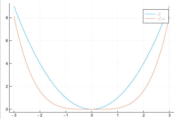
Such lines can be useful in the design of graphs.
x = [-3:0.1:3...]
y1 = x .^2
α = 10
y2 = x .^4 / α;
plot(x,y1, lab = "\$x^2_i\$")
plot!(x,y2, lab = L"x^4_i/\alpha")
Latexify
A more functional package is Latexify ( Guide ). It is designed to generate LaTeX math from julia objects. This package uses Julia's homology to convert expressions to strings in LaTeX format. Latexify.jl provides functions for converting a number of different Julia objects, including:
- Expressions
- Strings
- Numbers (including rational and complex),
- Symbolic expressions from SymEngine.jl,
- ParameterizedFunctions and ReactionNetworks from DifferentialEquations.jl
as well as arrays of all supported types.
ex = :(x/(y+x)^2) # выражение
latexify(ex)

str = "x/(2*k_1+x^2)" # строка
latexify(str)

Array of heterogeneous elements:
m = [2//3 "e^(-c*t)" 1+3im; :(x/(x+k_1)) "gamma(n)" :(log10(x))]
latexify(m)
![$ \ left [\ begin {array} {ccc} \ frac {2} {3} & e ^ {- c \ cdot t} & 1 + 3 \ textit {i} \\ \ frac {x} {x + k_ {1}} & \ Gamma \ left (n \ right) & \ log_ {10} \ left (x \ right) \\ \ end {array} \ right] $](https://habrastorage.org/getpro/habr/formulas/3e4/438/451/3e4438451fca235086760eb3eb1bdc01.svg)
You can specify a function that displays formulas and copies them to the buffer in the form that is understandable to Habr:
function habr(formula)
    l = latexify(formula)
    res = "\$\$display\$$l\$display\$\$\n"
    clipboard(res)
    return l
end
habr(ex)
$$$display$$\frac{x}{\left( y + x \right)^{2}}$$display$$$
Keep in mind
latexify("x/y") |> display

latexify("x/y") |> print
$\frac{x}{y}$
Symengine
SymEngine is a package that provides symbolic calculations that you can visualize in your Jupyter with Latexify.
You can specify characters in lines and quotes ( quote):
julia> a=symbols(:a); b=symbols(:b)
b
julia> a,b = symbols("a b")
(a, b)
julia> @vars a b
(a, b)
Define the matrix and beautifully display it
u = [symbols("u_$i$j") for i in 1:3, j in 1:3]
3×3 Array{Basic,2}:
 u_11  u_12  u_13
 u_21  u_22  u_23
 u_31  u_32  u_33
u |> habr
![$ \ left [\ begin {array} {ccc} u_ {11} & u_ {12} & u_ {13} \\ u_ {21} & u_ {22} & u_ {23} \\ u_ {31} & u_ {32} & u_ {33} \\ \ end {array} \ right] $](https://habrastorage.org/getpro/habr/formulas/fd4/de4/0b6/fd4de40b6bf47172d16febafa99740ac.svg)
Suppose we have vectors
C = symbols("Ω_b/Ω_l")
J  = [symbols("J_$i") for i in ['x','y','z'] ]
h  = [0, 0, symbols("h_z")]
3-element Array{Basic,1}:
   0
   0
 h_z
which must be vector-multiplied
using LinearAlgebra
× = cross
latexify(J×h, transpose = true)
Full matrix calculations:
dJ = C*(u*J.^3)×h
latexify( dJ, transpose = true)
habr(ans)
а вот такой нехитрой цепочкой можно найти детерминант и отправить его на Хабр
u |> det |> habr

Рекурсивненько! Обратная матрица наверно посчитается сходным образом:
u^-1 |> habr
Спойлер Если хотите сделать больно Матжаксу своего браузера, поставьте минус вторую степень (квадрат обратной матрицы)
Кстати, SymEngine считает производные:
dJ[1] |> habr

diff(dJ[1], J[1]) |> habr

К слову, Джулия может использовать из LaTeX 'a не только формулы, но и графики. И если вы установили MikTex и уже скачали pgfplots, то с помощью соответствующего окружения его можно сдружить с Джулией, что предоставит возможность строить гистограммы, трехмерные графики, ошибки и рельефы с изолиниями, а потом это интегрировать в LaTeX документ.
На этом с формулами всё, но не с символьными вычислениями: у Джулии еще есть более сложные и интересные решения для символьной алгебры, с которыми мы обязательно разберемся как-нибудь в следующий раз.