Exploring OpenCV on StereoPi: Depth Map from Video

Today we want to share a series of examples in Python for OpenCV learners on the Raspberry Pi, namely for the dual-chamber StereoPi board. The finished code (plus the Raspbian image) will help you go through all the steps, starting with capturing a picture and ending with getting a depth map from the captured video.

Introductory

I must emphasize right away that these examples are for a comfortable immersion in the topic, and not for a production solution. If you are an advanced OpenCV user and have been dealing with raspberries, then you know that for full-fledged work it is advisable to code on a bite, and even use a raspberry GPU. At the end of the article, I will touch on the “bottlenecks” of the python solution and overall performance in more detail.

What are we working with

As an iron we have such a setup here:



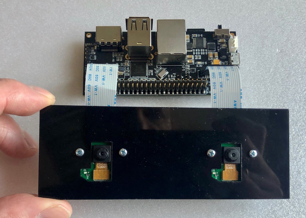
StereoPi board, on board the Raspberry Pi Compute Module 3+. The two simplest cameras are connected for the Raspberry Pi version V1 (on the ov5647 sensor).

What is installed:

• Raspbian Stretch (kernel 4.14.98-v7 +)
• Python 3.5.3
• OpenCV 3.4.4 (pre-compiled, 'pip' from Python Wheels)
• Picamera 1.13
• StereoVision lib 1.0.3 (https://github.com/erget/StereoVision)

The process of installing all the software is beyond the scope of this article, and we just suggest downloading the finished Raspbian image (links to the github at the end of the article).

Step one: capture a picture

To do this, use the 1_test.py script.

Open the console, go from the home folder to the folder with examples:

cd stereopi-tutorial

Run the script:

python 1_test.py

After starting, a preview of our stereo image is displayed on the screen. The process can be interrupted by pressing the Q button. This will save the last captured image, which will be used in one of the following scripts to configure the depth map.

This script allows you to make sure that all hardware is working correctly, as well as get the first picture for future use.

Here's what the first script looks like:

Step two: collect pictures for calibration

If we talk about a spherical horse in a vacuum, then to get a good quality depth map, we need to have two absolutely identical cameras, the vertical and optical axes of which are perfectly parallel, and the horizontal axes coincide. But in the real world, all cameras are slightly different, and it’s not possible to arrange them perfectly. Therefore, a software calibration trick was invented. Using two cameras from the real world, a large number of pictures of a previously known object are taken (we have a picture with a chessboard), and then a special algorithm calculates all the “imperfections” and tries to correct the pictures so that they are close to ideal.

This script does the first stage of work, namely it helps to make a series of photos for calibration.

Before each photo, the script starts a 5-second countdown. This time, as a rule, is enough to move the board to a new position, to make sure that on both cameras it does not crawl over the edges, and fix its position (so that there is no blur in the photo). By default, the series size is set to 30 photos.

Launch:

python 2_chess_cycle.py

Process:


As a result, we have a series of photos in the / scenes folder.

We cut pictures into pairs

The third script 3_pairs_cut.py cuts the photos taken into “left” and “right” pictures and saves them in the / pairs folder. In fact, we could exclude this script and do the cutting on the fly, but it is very useful in further experiments. For example, you can save slices from different series, use your scripts to work with these pairs, or even palm off pictures taken on other stereo cameras as pairs.

Plus, before cutting each image, the script displays its image, which often allows you to see failed photos before the next calibration step and simply delete them.

Run the script:

python 3_pairs_cut.py

Short video:


In the finished image there is a set of photographs and cut pairs that we used for our experiments.

Calibration

The script 4_calibration.py draws in all the pairs with the chessboards and calculates the necessary corrections to correct the pictures. In the script, automatic rejection of photographs on which a chessboard was not found was made, so that in case of unsuccessful photographs the work does not stop. After all 30 pairs of pictures have been uploaded, the calculation starts. It takes about a minute and a half with us. After completion, the script takes one of the stereo pairs, and on the basis of the calculated calibration parameters “corrects” them, displaying a rectified image on the screen. At this point, you can evaluate the quality of the calibration.

Run by command:

python 4_calibration.py

Calibration script in work:

Depth Map Setup

The 5_dm_tune.py script loads the picture taken by the first script and the calibration results. Next, an interface is displayed that allows you to change the settings of the depth map and see what changes. Tip: before setting the parameters, take a frame in which you will simultaneously have objects at different distances: close (30-40 centimeters), at an average distance (meter or two) and in the distance. This will allow you to choose the parameters in which close objects will be red and distant objects will be dark blue.

The image contains a file with our depth map settings. You can load our settings in the script simply by clicking the “Load settings” button.

Run:

python 5_dm_tune.py

Here's what the setup process looks like:

Real Time Depth Map

The last script 6_dm_video.py builds a depth map from the video using the results of previous scripts (calibration and setting of the depth map).

Launch:

python 6_dm_video.py

Actually the result:


We hope that our scripts will be useful in your experiments!

Just in case, I’ll add that all scripts have keystroke processing, and you can interrupt the work by pressing the Q button. If you stop “roughly”, for example, Ctrl + C, the process of Python interaction with the camera may break and a raspberry reboot will be required.

For advanced

• The first script in the process displays the average time between frame captures, and upon completion, the average FPS. This is a simple and convenient tool for selecting such image parameters in which the python is still not "choking". With it, we picked up 1280x480 at 20 FPS, in which the video is rendered without delay.
• You may notice that we capture a stereo pair in 1280x480 resolution, and then scale it to 640x240.
  
  A reasonable question: why all this, and why not immediately grab the thumbnail and not load our python by reducing it?
  
  Answer: with direct capture at very low resolutions, there are still problems in the raspberry core (the picture breaks). Therefore, we take a larger resolution, and then reduce the picture. Here we use a little trick: the picture is not scaled with python, but with the help of the GPU, so there is no load on the arm core.
• Why capture video in BGRA format, not BGR?
  We use GPU resources to reduce the size of the picture, and the native for the resize module is the BGRA format. If we use BGR instead of BGRA, we will have two drawbacks. The first is slightly lower than the final FPS (in our tests - 20 percent). The second is the constant worning in the console "PiCameraAlfaStripping: using alpha-stripping to convert to non-alpha format; you may find equivalent alpha format faster ”. Googling thereof led to the Picamera documentation section, which describes this trick.
• Where's the PiRGBArray?
  
  This is like the native Picamera class for working with the camera, but here it is not used. It has already turned out that in our tests, working with a “hand-made” numpy array is much faster (one and a half times) than using PiRGBArray. This does not mean that PiRGBArray is bad, most likely these are our crooked hands.
• How loaded is the percent in calculating the depth map?
  Let's answer with a picture:
  
  
  
  We see that out of 4 cores, only one is loaded, in fact, only 70%. And this despite the fact that we work with a GUI, and we are outputting pictures and depth maps to the user. This means that there is a good margin of performance, and fine tuning OpenCV with OpenMP and other goodies in C, as well as a “combat” mode without a GUI can give very interesting results.
• What is the maximum FPS depth map obtained with these settings?
  
  The maximum achieved by us was 17 FPS, when capturing 20 frames per second from the camera. The most “responsive” in terms of speed parameters in the depth map settings are MinDisparity and NumOfDisparities. This is logical, since they determine the number of "steps" performed within the algorithm by the search window for comparing frames. The second most responsive is preFilterCap; it affects, in particular, the “smoothness” of the depth map.
• What about the temperature of the processor?
  
  On Compute Module 3+ Lite (a new series, with an iron “cap” on the process) it shows roughly the following results:
  
  
• How to use GPU?
  
  At a minimum, it can be used for andistorization and rectification of pictures in real time, because there are examples ( here on WebGL ), Python Pi3d , as well as the Processing project ( examples for raspberries ).
  
  There is another interesting development by Koichi Nakamura, called py-videocore . In our correspondence with him, he expressed the idea that to accelerate StereoBM you can use its core and OpenCV sorts with Cuda support . In general, for optimization - an untouched edge, as they say.

Thank you for your attention, and here is the promised link to the source .