February 27, 2019 at 11:45
Game tornado physics: how aerodynamics are implemented in Just Cause 4 (traffic)
- Transfer
Jacques Kerner is a senior software engineer at Avalanche Studios.
As if the game wasn’t crazy enough before
The Just Cause and Avalanche Studios series of games are known for their open-world technology, providing a varied and exciting gameplay. The latest version of the game - Just Cause 4 - added wind and weather disasters, which became a novelty in the stack of technologies that deepen the gameplay. But extreme environmental conditions were originally conceived not just as a way to simulate a more believable world. The fury of nature is controlled by the forces of evil opposing Rico Rodriguez. We intended to make the wind manifest itself more clearly and extreme weather conditions did not look like sudden events alien to this world. This article presents the techniques developed by us to implement the wind in all its manifestations from a physical point of view, as well as the reaction of all objects to it.
[Under cat about 120 MB GIF files]
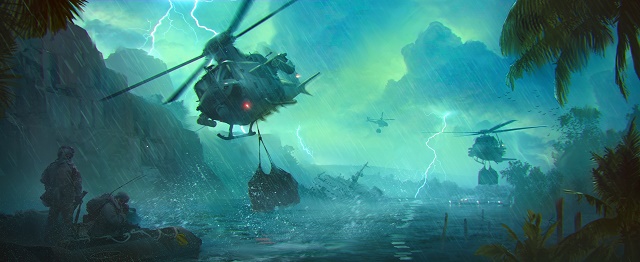
JC4 Tropical Storm - Early Concept (Volta)
As the development of Just Cause 3 was nearing completion, most of the team moved to the preproduction Just Cause 4, and the tiny kernel was left to work on patches for JC3 and downloadable content (“DLC”). Hamish Young and I, lead programmer and lead vehicle designer, focused on the Mech Land Assault DLC. We were supposed to be the leading designer of physics (and the mechanics of the player) and the leading programmer of physics JC4, but we were completely absorbed by the DLC at the time when the design of the new franchise series was being created, its attractive features and important functions were determined. This time a large-scale prototype was created to test the new basic mechanics and Rico's reaction to the wind. A draft of the plot was written, and the publisher Square Enix approved the initial development direction. The only thing left was to master the concept. But how to do that, without compromising performance? As soon as we started the project, we attacked the problem from two fronts: 1. set wide limits to avoid the worst-case scenarios (spoiler: we didn’t succeed) 2. dealt with various manifestations of extreme weather conditions, and in particular, hurricane winds, create a system that provides realistic behavior, but scales well to the desired number and density of objects.

Sandstorm in JC4 - Early Concept Art (Volta)
The bottleneck in real-time simulation, and especially open-world games, is the number of colliding physical bodies. The main expenses arise due to the calculation of collisions of many moving bodies colliding with each other and with a static environment (relief, buildings). That is why physical engines like Havok separate active and inactive bodies. Active bodies are checked for collisions with other bodies and require full computational cost. If the active body does not move for several frames, then the physical engine marks it as inactive, and from that moment it can be completely ignored until it is “woken up” by the approaching active body. Such inactive bodies usually rest on the ground and collision checks between them and the earth are no longer performed. Obviously that the ubiquitous presence of wind in the open world will become a threat to this system, so it was important for us to ensure that the wind remained moderate and purely cosmetic when exposed to large areas, or strong and physically activating when occurring in small volumes and places where the number of potentially active bodies are small. I talked about these limitations to our design department in the early stages of development so that it would not be trapped. At first, it seemed that the designers had listened and decided to limit the trajectories of extreme weather events to predetermined destruction routes, within which more stringent rules for building the world should apply. And they did observe some of these restrictions. But the temptation was too great, and the pressure of colleagues who wanted to make the game as good as possible, proved insurmountable. What was I just thinking? Immediately after that, the designers created a tornado several kilometers high, passing right through the capital of the country - the most densely populated part of the island. This tornado boldly not only half the capital, but also some of the unsuspecting programmers who did not adhere to this basic feature of the game too strictly.
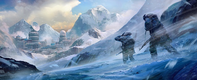
Blizzard in JC4 - Early Concept Art (Volta)
In general, extreme weather physics at JC4 required the following ingredients:
These three problems needed to be solved simultaneously, and as soon as possible. Many design decisions depended on the possibility of implementing all three aspects, and during the first months we felt dissatisfied with the designers who patiently waited for the opportunity to play around with the system on a large scale.
First, we created a model of aerodynamic drag. After its completion, each object suddenly learned to respond in a fairly realistic way to the wind. For example, if any object falls off a cliff or is thrown off by an explosion, all objects slow down and realistically rotate in the air, which in itself was already worth the effort. But in the absence of wind sources, it was difficult to say how they would behave in conditions of extreme wind. Although we were proud of ourselves and the fact that experience and intuition helped us quickly find an approach to the first two problems that met the performance requirements, we decided that we were very lucky when the first version of the tornado started working exactly as we expected. She lifted all the dynamic objects and twisted them in a rather realistic way, without taking up all the processor time. JC4 director Francesco Antollini, who very often asked about the tornado situation, appeared right next to my workstation and expressed his relief: I think I missed the opportunity to shame him for doubting me; but actually I felt the same way.
From a physical point of view, JC4 was a breakthrough compared to JC3: it is a more dense, filled, vibrant and beautiful world, which is much more interesting to destroy. And all this was possible on the same target platforms (XBox One and PlayStation 4). Not surprisingly, optimization took a very long time. Our technical director Dave Barrett immediately took advantage of our advantage: we had the necessary performance indicators for JC3, so the head of the engine development department, Daniel Pieroni, was given the task to determine what maximum costs of performance and memory can be used for each technical aspect. We were given physics a generous 8.5 ms on 4 threads out of 33 ms processor time, allocated to create a frame with a frequency of 30 times per second. Havok occupied a large part of this budget for recognizing possible collisions between objects, calculating contacts, resolving constraints, and “integrating” the movement of all active bodies to determine their position after 33 ms of simulated time. I roughly calculated that our budget for all calculations related to aerodynamics and wind should be approximately 1 ms on 4 threads. Basically, we managed to stay within the budget, although it is most likely better to ask Daniel about this. The solution presented below is fast enough for real time when calculating several hundred objects on modern CPUs. Of course, it, like much more, can be further optimized by adapting it to work on the GPU. resolution of restrictions and "integration" of the motion of all active bodies to determine their position after 33 ms of simulated time. I roughly calculated that our budget for all calculations related to aerodynamics and wind should be approximately 1 ms on 4 threads. Basically, we managed to stay within the budget, although it is most likely better to ask Daniel about this. The solution presented below is fast enough for real time when calculating several hundred objects on modern CPUs. Of course, it, like much more, can be further optimized by adapting it to work on the GPU. resolution of restrictions and "integration" of the motion of all active bodies to determine their position after 33 ms of simulated time. I roughly calculated that our budget for all calculations related to aerodynamics and wind should be approximately 1 ms on 4 threads. Basically, we managed to stay within the budget, although it is most likely better to ask Daniel about this. The solution presented below is fast enough for real time when calculating several hundred objects on modern CPUs. Of course, it, like much more, can be further optimized by adapting it to work on the GPU. although it’s probably best to ask Daniel. The solution presented below is fast enough for real time when calculating several hundred objects on modern CPUs. Of course, it, like much more, can be further optimized by adapting it to work on the GPU. although it’s probably best to ask Daniel. The solution presented below is fast enough for real time when calculating several hundred objects on modern CPUs. Of course, it, like much more, can be further optimized by adapting it to work on the GPU.
In the remainder of the article, I will briefly talk about how we solved each of the problems, and for those who are interested, I will present in the applications details and mathematical calculations.

Wind in JC4 - Early Concept Art (Ironklad Studios)
Our goal in creating the model of resistance was to evaluate the forces of resistance and torques, which would approximately resemble those that are applied to a body of arbitrary shape in the real world. Notice how unambitious we were here - no one demanded huge realism. However, we had some requirements. Firstly, the resistance forces must counteract the movement of the body. Secondly, the force must be calculated from the basic equation of aerodynamic drag, i.e. vary in accordance with the surface area of the figure and the square of the speed of movement through the air. Finally, somehow the shape and size of the body must be taken into account so that objects with the same surface area but very different shapes behave differently. I was tempted to simply approximate the shape of each body according to the parallelogram that describes it, but I thought that something more was needed, because it was obvious - the shape of many objects can differ significantly from a box or even a small number of boxes. My previous experience working with systems that roughly approximate the volume of 3D objects using voxels or spheres made me look for a better solution. I was offered to select resistance coefficients for each object manually, but I wanted to avoid one more stage of manual adjustment in an already complicated pipeline. Therefore, I continued to search for an automated way. And I'm glad I did not back down. My previous experience working with systems that roughly approximate the volume of 3D objects using voxels or spheres made me look for a better solution. I was offered to select resistance coefficients for each object manually, but I wanted to avoid one more stage of manual adjustment in an already complicated pipeline. Therefore, I continued to search for an automated way. And I'm glad I did not back down. My previous experience working with systems that roughly approximate the volume of 3D objects using voxels or spheres made me look for a better solution. I was offered to select resistance coefficients for each object manually, but I wanted to avoid one more stage of manual adjustment in an already complicated pipeline. Therefore, I continued to search for an automated way. And I'm glad I did not back down.
The simplest way to evaluate the wind pressure on each surface of the collision shape of our objects is to take into account only the incoming wind, ignoring all air circulation around the objects and the viscosity of the air surrounding them. As if the air resistance consists only of moving forward the mass of air in front of the object or its absorption on the other hand. An early prototype showed that this method was good enough for our purposes.
The “only” problem was that the sum of the contributions of thousands of triangles for each individual figure during the execution of the game was an order of magnitude higher than the required cost level. In "heavy" scenes, we could easily reach more than 100,000 faces. It would be great if we could calculate the forces in advance. The first method of “brute force” consisted in a preliminary calculation of the aerodynamic forces and torques that arise when a body moves at different speeds in several directions in still air when it rotates at different angular speeds in different directions. So we got a lookup table from which we could take values during the execution of the game. This can be thought of as a virtual wind tunnel, included during the compilation of our content,
What will this table look like? The known values at runtime are the linear and angular velocity of the body, therefore , that is, only about 300 KB per object. And still, this is at least an order of magnitude greater than the allowable memory consumption.
To significantly reduce the number of samples, I used two techniques. Firstly, I converted the calculation to a linear form into a sum of contributions based on preliminary calculation of forces and torques separately for only a moving and only rotating body. Secondly, I approximated this into an analytical formula for extrapolating values at arbitrary speeds based on a pre-calculated reaction and only at a speed of 1 m / s and a speed of 1 rad / s. This reduced the pre-computed table to just 7 KB per object. Unfortunately, for this I had to perform several approximations. The reason for the problem is that even with a very simple model of resistance, we are faced with the fact that the forces applied to the body, that is, rotation and displacement is not just the sum of the applied forces individually for rotation and displacement. Even though I had to add approximations, I managed to save some of the terms caused by a combination of rotation when moving, similar to the Coriolis component. The conclusion of the wording can be found in Appendix 1. As a result, instead of directly storing the forces and torques for each sample, we store the vector of members used in the linear formulas. Each sample corresponds to a unit linear velocity relative to air at 1 m / s or a unit angular velocity relative to air at 1 rad / s, in a certain direction. The components of this vector are used in the formula, which also takes into account the true linear and angular velocities of the object relative to the air when calculating the forces and torques that need to be applied to the object. Appendix 1 details how this happens.
To store the search table, we used a cube map, i.e. a cube whose faces are divided into grids of size, say 3x3 cells, like a Rubik's cube. We store values in the corners of the cells, so each face can store 4x4 values. In each corner of the cell, we calculate the vector going from the center of the cube to the corner, and normalize this vector to get the unit direction. We use this unit direction vector asfor the corner of the cell. As a result, we get 6 tables (one per edge) of 16 elements with 19 float values each, which is slightly more than 7 KB, and this is very convenient. There are ways to further reduce the number of samples, but with this method it is very easy to interpolate the direction of arbitrary speed: since it always falls into the cell, it is always possible to use the values in the four corners of this cell to perform bilinear interpolation for this specific direction. The technique of cubic maps and bilinear interpolation is very widely used in rendering, so finding information about it and the corresponding code is very easy.
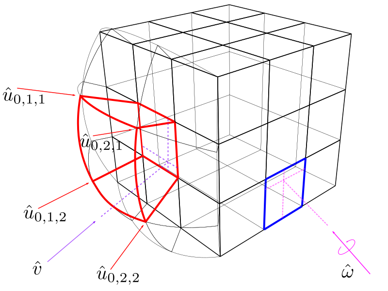
Figure 1. Cubic map of unit velocities relative to air. In this figure, I highlighted in red a separate cell of a cubic map to illustrate the principle. Having linear speed relative to air, we again sample the same cubic map to find the blue cell and use the 4 coefficients stored in its corners. Then we mix all the values according to the formula in Appendix 1.
Although in most cases this worked, we ran into difficulties in changing the center of mass or the scale of objects at runtime. Our solutions to these problems can be found in Appendices 2 and 3.
When developing this model, I was not sure about the number of samples sufficient to get good behavior of objects moving and rotating in the air, so I didn’t know exactly if I had enough memory on the disk at runtime. In parallel, we began to create new destruction assets for Havok, with hundreds of fragments of various sizes, sometimes several hundred parts for one asset. It dawned on me that some of these assets would require the same amount of memory, as many other assets in total, if each fragment had its own cubic map. The general model well conveyed some unique characteristics of complex objects, but was too much for small fragments. In addition, I was not sure about the cost at runtime, and being able to return to a lower cost model was a good way to reduce risk. Therefore, I found a very compact wording (making generous approximations) based only on bounding boxes of objects. It can be found in Appendix 4.
We introduced the concept of wind volumes, supporting the idea that a strong, physically activating object wind can occur only in finite spaces, and began to classify them according to the shape and distribution of the wind. We divided the wind volumes into the following main types:
This restriction of the wind by the final volume was criticized several times, and at the last moment they almost abandoned it, replacing it with a “topographic wind”. The wind everywhere was supposed to correspond to the movement of clouds in the upper atmosphere and provide the player with an upward flow of air when meeting with an increasing slope of the terrain. We implemented it, but the lack of a clear graphic display of the wind forced us to abandon this function. The guys from the rendering department already had too many tasks for implementing clouds, rivers, waterfalls, upgrading to DirectX 12 and much more.
In retrospect, it turned out that storms became the simplest volumes of wind, both in terms of shape (cylinder) and wind distribution (almost unidirectional for a sandstorm, or rotating around a central axis for a blizzard). On the other hand, tornadoes and wind tunnels turned out to be more complex and deserve a more detailed explanation.
We had a clear and simple idea of how objects should rotate around a tornado, but we did not agree on the distribution of winds necessary to achieve this result. Instead of endless debate, we made the various components of the wind field customizable at runtime so that Hamish could experiment with them and quickly find a working option. A tornado is essentially a stack of horizontal cylinders whose centers are located on the central spline, which deforms over time. In these horizontal cylinders, we decomposed the tornado wind field into cylindrical coordinates with a tangent component, a radial component, and a vertical component. Each component can be adjusted using variable curves.

Figure 2. Our majestic tornado - shaders were created by Gabriel Sassone. Engin Silasun, Stephen Ewan, Eddie Gong and Hamish Young. All of them contributed at different stages of development. Time is accelerated unevenly to show you a beautiful picture during the day and skip the night stages.
As with many other features, and as is often the case in our industry, Hamish and I often went from setting to code until the result was good enough. Hamish tweaked the curves to his liking, throwing dozens of 12-meter containers along the tornado to look at their behavior. He used the maximum recorded wind speed (about 230 mph) for the tornado. After some time, Hamish discovered that his setup was becoming more complicated, because it was necessary to make the wind everywhere correspond to a simple rotational motion, but at the same time attracted objects to the center. Angular velocity was already part of the field, not only pushing, but also rotating objects in a tornado. This ensured that, for example, objects stuck in the center would rotate in place, as we wanted. Therefore, Hamish asked to start with the wind, everywhere corresponding to this angular velocity in the center, that is, start with the velocity field of an ideal rotation field, into which a custom wind field can be added. After this last setup, the curves began to consist of the following components:
Where - the height above the bottom of the tornado, and
  - distance from the center. The tornado wind speed is given by the equation:
When objects are accelerated to the tangent speed of the tornado at a given distance, the tangent component of the air resistance forces is essentially zero, because both the air and the object move in tangent in unison. The remainder of the wind speed draws the object inward, as the planet attracts satellites to bend its trajectory so that it remains in orbit; Also, objects are pushed up to reach greater heights. Pushing objects up is the most important performance optimization, preventing costly calculations of the contacts of hundreds of objects and the earth. It also helps that with the height of the tornado it increases the radius by spatially distributing objects to reduce the likelihood of their collision and contact calculation. A tornado in the real world is formed by the exchange of air when a layer of cold air is on top of a layer of warm air. Warm air rises up like a whirlpool around the center of a tornado, which is cold air coming down. Therefore, in principle, in the center of the funnel, the wind speed should be strongly directed downward. As you can see, this is not implemented in our country to reduce the likelihood of pushing objects down to the ground and pulling them into a tornado, otherwise this would increase the costly calculation of collisions.
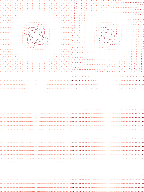
Figure 3. Tornado wind field in a horizontal section (above), and in a vertical section (below). Two cuts on the left do not account for a member the rotating field of the wind with which we started, in order to better understand whether an additional field is necessary for the proper operation of the tornado. In the version on the right, a rotating field is added. In the distance we see a very fast wind, at any point directed at about 45 degrees from the radius. The vertical section on the left shows how much the tornado should pull into the center. Then there is a small transition interval in which there is almost no wind, and behind it there is a strong rotating field in the center. The strength of the wind field is shown in color, the redder, the stronger.

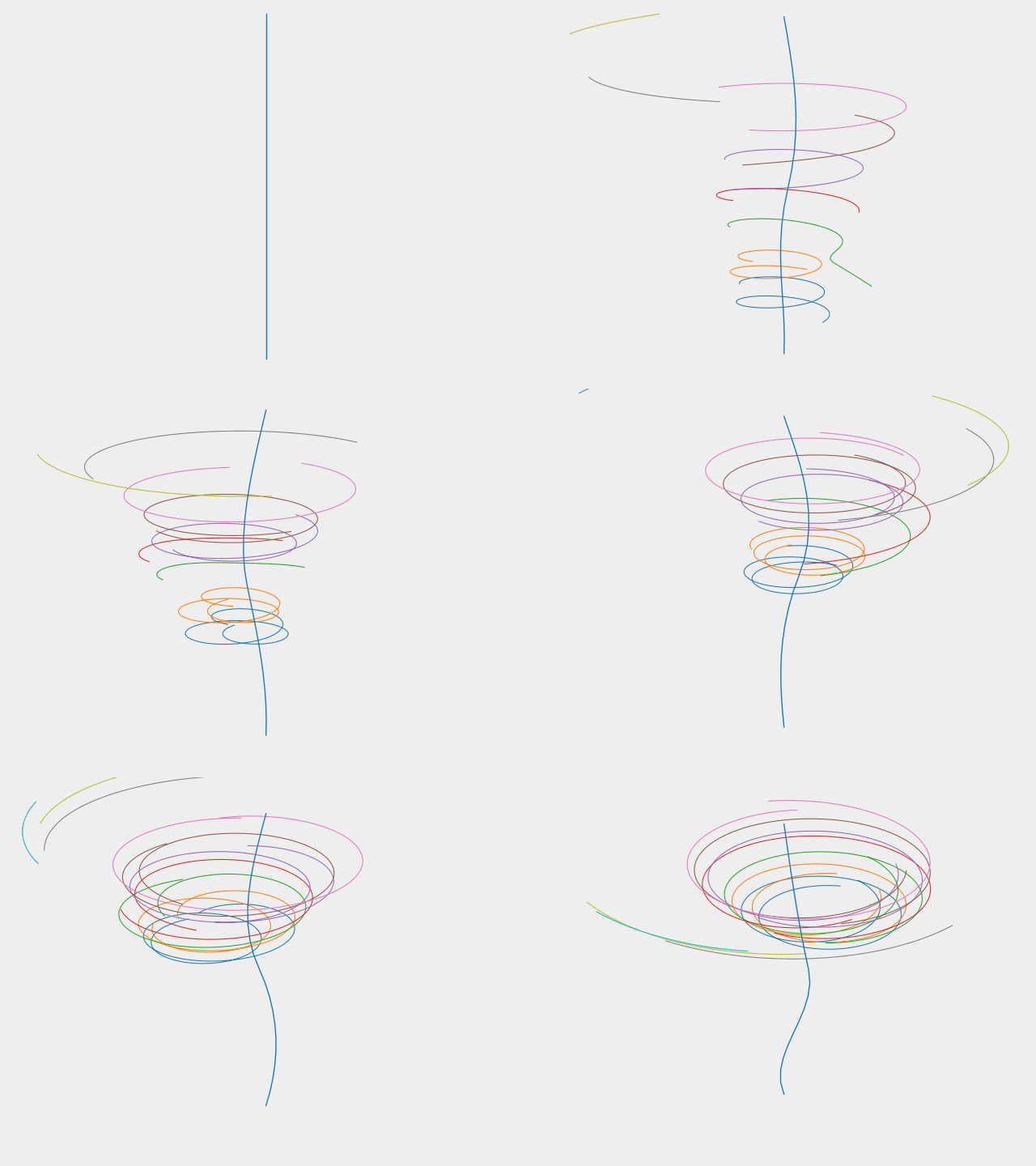
Figure 4. Lines of the paths around the tornado wind field - the central spline of the line.
A direct tornado seems boring. To deform it, we used 2 cubic splines connected by the ends, 3 control points of which are in orbit and move at different speeds around an imaginary vertical line. The resulting tornado profile changes over time, so it slowly shifts from the S-shape to the C-shape, and vice versa. Appendix 5 details how we created splines. Interestingly, the tornado in warped mode didn’t work as well. Objects circling in the orbit of a direct tornado now scattered as soon as the central split of the tornado moved away from them, and sadly fell to the ground. To fix this problem, we added another term to the speed due to the deformation of the tornado itself. In the end, this deformation should primarily occur due to air movement, and it seemed natural to us to add this component. This solved the problem beautifully, giving us path lines very similar to the picture below.
Figure 5. Lines of paths around the tornado wind field - the central spline bends over time
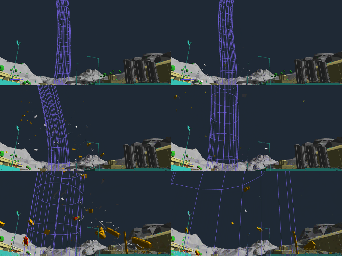
Figure 6. An example of a tornado in a game, it destroys and absorbs everything in its path. This is the Havok Visual Debugger (VDB), an extremely useful tool that allows us to observe simulated elements.
Wind tunnels have been designed to provide physical wind control in parts of the world, such as canyons and caves, as well as smoke columns in front of huge industrial fans and wind cannons. They can be used to guide the player in certain spaces or missions. Our first prototypes used a traditional cylinder with a uniform vector field of constant speed parallel to the axis of rotation of the cylinder. Placing all these cylinders in the scene was a painstaking task, so instead we used a cubic Bezier spline around which a circle of varying radius is stretched. This shape is approximated by dividing the central spline into capsule-shaped figures, i.e. on capsules with different radii around the edges. The velocity field in them has also undergone some changes. Initially, the wind in the tunnel was tangent to the central spline. We set the wind speeds at each control point of the spline, and they were interpolated from one control point to another along a spline segment. However, Joshua Espinosa (the designer who worked on the wind tunnels and the player’s movements on them) soon found out that he needed two more components. One component is the upstream, giving the player an additional artificial lift, always pointing up. We called the other component “retraction”, it pushes the player towards the center spline, but most of all at the edges of the tunnel, dropping to the center to zero. Finally, the reduction boundary in the outer part of the tunnel ensured a smooth transition from the outer to the outer part of the tunnel. The thickness of this boundary is specified as a percentage of the radius; it acts along the entire wind tunnel.

Figure 7. Wind tunnel divided into a sequence of overlapping capsule-shaped figures. Separation occurs when the direction of the spline changes, or when it is no longer possible to perform linear longitudinal interpolation of radius (A) or wind speed (B). We calculated the second derivative of these variables along the spline to determine when to split.

Figure 8. Wind tunnels edited in the Apex Engine. The wind tunnel is broken into capsules in the right way, depending on the spline, changes in the radius and speed of the wind along the spline. As stated in the next section, you can also see the spatial separation that sorts the capsule-shaped figures into Morton curves. These calculations are fast enough for real-time updates; in addition, you can quickly interact with the wind tunnel to test it. The editing tool was made by reworking some parts of the river creation tool with the addition of debugging rendering.
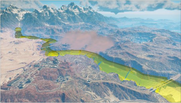
Figure 9. An example of a long wind tunnel allowing a player to move upstream to a mountain. The river current pushes Rick to the sea, and the wind can quickly return him inside the land on top of the same river. The player’s mechanics department noticed that Rico’s side winds were too sharp, so the main influence of the wind is to accelerate the player (with a fair wind) or to brake (headwind) and give him an additional lift (upstream component).
Figure 10. Rico in wingsuit in the same wind tunnel. Here the player did not control the direction. At first, Rico loses altitude until it reaches the outer part of the wind tunnel, which gradually slows its decline. Then the central part creates sufficient upward flow to overcome gravity and quickly accelerates it up the canyon. The JC3 Wingsuit code for proper interaction with the wind was developed by Joshua Espinosa, Hamish Young and Rickard Granfeld.
With the potential for hundreds of active bodies, calculating the local wind in their position should be a quick process. We started optimizing the queries by calculating the AABB (axis aligned bounding box) for each wind volume and storing them in a tightly packed array. This allows brute-force rejection because it is possible to quickly check the position with respect to each AABB without cache misses. In each AABB frame, the wind volumes in the array are updated to prepare for the request.
If the position is inside the volume of the storm, then we directly calculate the effect of the wind using a cylindrical shape. For a tornado, you need to do more calculations, because at the top it is much wider than at the bottom, while the highest density of objects is at the bottom. The AABB solution doesn’t very well cut objects near the tornado, so we used cylinders stacked on top of each other. They transmit the tornado shape much closer and are used to clip objects before calculating the wind. The latest tornado optimization was to avoid projecting the query position onto the central spline. This was possible because although the spline tornado is interpolated in 3D points, it is therefore a parametric 3D curve, in practice, the control points interpolated by him are uniformly and sequentially distributed along the vertical, which gives us a fairly simple curve. In general, projecting a point onto a 3D spline or finding a point on that spline with the same height requires a search along that spline. But instead, we decided to change the way the spline is sampled using the height above the bottom of the tornado as a sampling parameter for the spline itself. This slightly changes the shape of the spline, but the spline still passes through the interpolation points. But at the same time, to find a point on the spline at the same height, it comes down to transferring the height of the request position to it, followed by fixing the height of the point in the height of the request. For control points located unevenly along the vertical axis, the difference is noticeable, but when they are evenly located, it is barely visible.
Wind tunnels also required optimization, because the projection of each query point on the central spline of each wind tunnel was not even considered. Fortunately, we managed to take advantage of the technology simultaneously implemented for the rivers by Engin Silasun: a sparse spatial database. We divide the space into 32 . If the cell is not in the spatial database, then there is no wind at the query point caused by wind tunnels. If the cell is found, then you need to perform a more expensive check. In addition, this check should be fairly quick, and so we cut the wind tunnels to capsule-shaped figures. In the general case, capsules are used because it is possible to calculate the distance to their central segment at low cost. Capsule-shaped figures are a bit more expensive, but still faster than finding the shortest distance to a cubic spline. Another property of a spatially holistic system of wind tunnels is that we can remember the cell index of a certain object located in the previous frame and use it as a hint to speed up the query in the next frame,

Figure 11. Capsule-shaped figures of wind tunnels are entered into a sparse spatial database in accordance with the cells that they cross. The result is an array of 9 cells, each of which has only a few capsule-shaped figures.
The combination of the techniques we used has proven to be highly effective. By themselves, these techniques are actively used in programming. Most of the work lies in their selection and ensuring their proper collaboration to solve the current problem. This is typical for programming video games: it is full of small problems that require simple but reliable solutions.
The model of air resistance is extremely simplified and does not reflect some important properties of the real fluid flow. For example, a sheet at an angle of 45 degrees will generate more lift than in our rough model. But the good thing about it is that forces and torques are not calculated at runtime, and a solution with a cubic map avoids a more detailed simulation. In fact, we checked the calculations of forces and torques generated on the entire cubic map of the test object (a vintage car from JC4) using open source computational fluid dynamics software (OpenFOAM). The comparison showed that we were not too far removed from the correct results, but the “shape” of the cubic maps was different, and I expect that it will differ even more for objects in the shape of a wing. However, it took several hours to calculate the software, therefore, it is obvious that such a solution is not suitable for use on all objects. Our method took less than a second per object. But I think it would be very interesting for physics-based games to have fast, but realistic aerodynamic coefficients for all objects. Suppose Rico could collect objects in huge boomerangs. I briefly played around with this idea, watching the fast fall and rotation of maple helicopter seeds, and created a model in Maya to see what happens. The result turned out to be better than expected, and the object really rotated slowly when it fell. But it seems to me that for faster rotation it will be necessary to significantly improve the model of air resistance. As often happens, we simply did not have enough time. Our method took less than a second per object. But I think it would be very interesting for physics-based games to have fast, but realistic aerodynamic coefficients for all objects. Suppose Rico could collect objects in huge boomerangs. I briefly played around with this idea, watching the fast fall and rotation of maple helicopter seeds, and created a model in Maya to see what happens. The result turned out to be better than expected, and the object really rotated slowly when it fell. But it seems to me that for faster rotation it will be necessary to significantly improve the model of air resistance. As often happens, we simply did not have enough time. Our method took less than a second per object. But I think it would be very interesting for physics-based games to have fast, but realistic aerodynamic coefficients for all objects. Suppose Rico could collect objects in huge boomerangs. I briefly played around with this idea, watching the fast fall and rotation of maple helicopter seeds, and created a model in Maya to see what happens. The result turned out to be better than expected, and the object really rotated slowly when it fell. But it seems to me that for faster rotation it will be necessary to significantly improve the model of air resistance. As often happens, we simply did not have enough time. Rico could collect objects in huge boomerangs. I briefly played around with this idea, watching the fast fall and rotation of maple helicopter seeds, and created a model in Maya to see what happens. The result turned out to be better than expected, and the object really rotated slowly when it fell. But it seems to me that for faster rotation it will be necessary to significantly improve the model of air resistance. As often happens, we simply did not have enough time. Rico could collect objects in huge boomerangs. I briefly played around with this idea, watching the fast fall and rotation of maple helicopter seeds, and created a model in Maya to see what happens. The result turned out to be better than expected, and the object really rotated slowly when it fell. But it seems to me that for faster rotation it will be necessary to significantly improve the model of air resistance. As often happens, we simply did not have enough time. for faster rotation, it will be necessary to significantly improve the air resistance model. As often happens, we simply did not have enough time. for faster rotation, it will be necessary to significantly improve the air resistance model. As often happens, we simply did not have enough time.
Figure 12. Left: all orientations of a vintage oil car from Just Cause 4, placed in a virtual wind tunnel to fill a cubic map with a 5x5 grid on each face. Right: Paraview visualized results for two orientations - at an angle above (above) and behind (below). Red indicates high pressure, blue indicates low pressure, lines indicate flows.
Tornadoes and storms worked very effectively. Tornado deformation can still be improved. If we spent more time on this, we would probably be able to make water tornadoes (of course, with sharks instead of cows), whirlpools or fiery tornadoes. We had another idea - to develop a cannon that creates a mini-tornado.
Wind tunnels have been used in different parts of the world to control wind on an island, such as canyons, missions, around some military bases. They help the player cross the vast expanses of our open world with strategically located rising winds. But I think it would be better to use the idea of topographic wind, which we did not have time to implement. It would be more rational to implement it first, it would give us a systematic all-pervasive wind that almost does not require adjustment, and wind tunnels would provide local control over deviations from it.
And, finally, it was a logical idea to use wind barriers as game mechanics. We implemented a playable prototype of obstacles, which was shown inside the team, but abandoned it due to lack of time for the correct implementation. His physics was only part of the total cost of this feature, which was supposed to be supported by most of the development team.
But nothing can distract me from how proud I am of what we managed to do in JC4. Our visualization of extreme weather conditions and in particular tornadoes, combined with Rico’s ability to move in space, made it possible to create an absolutely unique and outstanding gameplay. I hope you enjoyed playing JC4 as much as we did when we created it.

We view the body defined by the mesh
 ![$ T_i, i \ in [0, N-1] $](https://habrastorage.org/getpro/habr/formulas/95a/e93/c72/95ae93c7289e9aa62576fe66c0d06549.svg) .
.
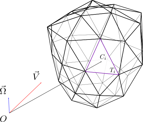
Figure 13. The body![$ i \ in [0, N-1] $](https://habrastorage.org/getpro/habr/formulas/ab3/d0b/fec/ab3d0bfecd9e8317c65bfbeb918d3dfe.svg) .
.
Consider a triangle :
:
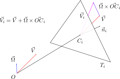
Figure 14. Triangle and speed in its center.
Now we need to write elemental force acting on this triangle. It is here that we need to take into account our requirements:
This complies well with the requirements, because the force is almost always directed to the side against the direction of movement, proportional to the surface area of the triangle and proportional to the square of the speed of the triangle relative to air. To get the force acting on the whole body, it is enough for us to summarize these forces:
As we strive to reduce everything to 1 m / s and 1 rad / s, let's rewrite with:
And now the first big approximation:
This is equivalent to approximating the length of the hypotenuse of a triangle by the sum of the lengths of its two sides. This approximation is also known as “city block distance” (Manhattan distance). When I was working on this task, I was just in Manhattan, so it would be foolish not to use it. So we have the following:
We decompose:
At first, this may seem intimidating. But then you notice that this is what we were looking for. Note that only amounts are found with its average value among all triangles:
Let's denote it by. Now we can finally write:
Where:
Moment of these forces relative to the point can be obtained in a similar way. And as a result, we get the following:
Where:
Given the above definitions, we can now form a vector:
This is a vector of 19 values and we refer to the sample table , but we can find fairly close values, and then either use them directly, or use them to interpolate the output. And at this stage, the cubic map described in the article comes into play.
You may notice that the values shown above are calculated relative to an arbitrary point . The total force acting on the body is simply the sum of all the forces:
Moments are set as:
and the total moment of these forces relative to the point is equal to:
Now it’s just a mathematical definition, a formula that cannot be used directly to change the movement of the body, because the center of gravity in this formula, according to the Schall theorem, is equal to:
We recognize the moment of forces with respect to , so:
, so:
And it is very useful for us if we calculated the total strength unchanged and applied the following torque to the center of mass:
At first, I decided to just take the origin of the body as a point in the center of the bounding parallelogram of the body, which should still be close to the center of mass and localized wind sampling in the most logical place relative to the body.
Another flaw appeared when balloons were introduced into the game. These balls are spherical bodies, the size of which can vary with a factor of 5 or 10. As in the case of the center of mass, it was too costly to recalculate the aerodynamic properties at run time. Is it possible to derive an analytical formula?
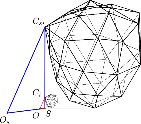
Figure 15 Body
Consider the body againbut now for a scaled object. We get:
Using the same approximations as the first time, and replacing , we get:
For the center of mass of the scaled body .
.
There are many ways to approximate forces and torques for a parallelogram, and different formulas can be obtained. Compact enough, easy to implement in code and calculations at runtime, it can be inferred by ignoring the effect of angular motion on linear force and the effect of linear speed on torque. Taking bounding parallelogram size , we can come to the following compact formulas:
The tornado is centered around a central curve whose shape is slowly changing. We implemented this using two consecutive Bezier cubic splines: for the bottom and
  for the top. Spline has control points
  ,
,  ,
,  and
and  , a controlled by points
  ,
,  ,
,  and
and  . The position of the tornado itself is at a point on the ground and the highest point It starts right above the level of the cloud layer, but is late in time, slowly following the position on the earth. Since the curves are connected at one end, and coincide in space. We also used 3 horizontal reference orbits for points, and . Finally, was located exactly at the midpoints between and , a at the midpoint between and .
As if the game wasn’t crazy enough before
Introduction
The Just Cause and Avalanche Studios series of games are known for their open-world technology, providing a varied and exciting gameplay. The latest version of the game - Just Cause 4 - added wind and weather disasters, which became a novelty in the stack of technologies that deepen the gameplay. But extreme environmental conditions were originally conceived not just as a way to simulate a more believable world. The fury of nature is controlled by the forces of evil opposing Rico Rodriguez. We intended to make the wind manifest itself more clearly and extreme weather conditions did not look like sudden events alien to this world. This article presents the techniques developed by us to implement the wind in all its manifestations from a physical point of view, as well as the reaction of all objects to it.
[Under cat about 120 MB GIF files]
JC4 Tropical Storm - Early Concept (Volta)
An offer we could not refuse
As the development of Just Cause 3 was nearing completion, most of the team moved to the preproduction Just Cause 4, and the tiny kernel was left to work on patches for JC3 and downloadable content (“DLC”). Hamish Young and I, lead programmer and lead vehicle designer, focused on the Mech Land Assault DLC. We were supposed to be the leading designer of physics (and the mechanics of the player) and the leading programmer of physics JC4, but we were completely absorbed by the DLC at the time when the design of the new franchise series was being created, its attractive features and important functions were determined. This time a large-scale prototype was created to test the new basic mechanics and Rico's reaction to the wind. A draft of the plot was written, and the publisher Square Enix approved the initial development direction. The only thing left was to master the concept. But how to do that, without compromising performance? As soon as we started the project, we attacked the problem from two fronts: 1. set wide limits to avoid the worst-case scenarios (spoiler: we didn’t succeed) 2. dealt with various manifestations of extreme weather conditions, and in particular, hurricane winds, create a system that provides realistic behavior, but scales well to the desired number and density of objects.
Sandstorm in JC4 - Early Concept Art (Volta)
Damage control
The bottleneck in real-time simulation, and especially open-world games, is the number of colliding physical bodies. The main expenses arise due to the calculation of collisions of many moving bodies colliding with each other and with a static environment (relief, buildings). That is why physical engines like Havok separate active and inactive bodies. Active bodies are checked for collisions with other bodies and require full computational cost. If the active body does not move for several frames, then the physical engine marks it as inactive, and from that moment it can be completely ignored until it is “woken up” by the approaching active body. Such inactive bodies usually rest on the ground and collision checks between them and the earth are no longer performed. Obviously that the ubiquitous presence of wind in the open world will become a threat to this system, so it was important for us to ensure that the wind remained moderate and purely cosmetic when exposed to large areas, or strong and physically activating when occurring in small volumes and places where the number of potentially active bodies are small. I talked about these limitations to our design department in the early stages of development so that it would not be trapped. At first, it seemed that the designers had listened and decided to limit the trajectories of extreme weather events to predetermined destruction routes, within which more stringent rules for building the world should apply. And they did observe some of these restrictions. But the temptation was too great, and the pressure of colleagues who wanted to make the game as good as possible, proved insurmountable. What was I just thinking? Immediately after that, the designers created a tornado several kilometers high, passing right through the capital of the country - the most densely populated part of the island. This tornado boldly not only half the capital, but also some of the unsuspecting programmers who did not adhere to this basic feature of the game too strictly.
Blizzard in JC4 - Early Concept Art (Volta)
General approach
In general, extreme weather physics at JC4 required the following ingredients:
- Aerodynamic drag model applied to all dynamic objects of the world, taking into account their shape and size
- Wind sources that correspond in shape and distribution to extreme weather conditions (storm, tornado), but also provide patterns of wind propagation around the world
- Optimization of the above systems so that the game fits into the budget of computing loads
These three problems needed to be solved simultaneously, and as soon as possible. Many design decisions depended on the possibility of implementing all three aspects, and during the first months we felt dissatisfied with the designers who patiently waited for the opportunity to play around with the system on a large scale.
First, we created a model of aerodynamic drag. After its completion, each object suddenly learned to respond in a fairly realistic way to the wind. For example, if any object falls off a cliff or is thrown off by an explosion, all objects slow down and realistically rotate in the air, which in itself was already worth the effort. But in the absence of wind sources, it was difficult to say how they would behave in conditions of extreme wind. Although we were proud of ourselves and the fact that experience and intuition helped us quickly find an approach to the first two problems that met the performance requirements, we decided that we were very lucky when the first version of the tornado started working exactly as we expected. She lifted all the dynamic objects and twisted them in a rather realistic way, without taking up all the processor time. JC4 director Francesco Antollini, who very often asked about the tornado situation, appeared right next to my workstation and expressed his relief: I think I missed the opportunity to shame him for doubting me; but actually I felt the same way.
From a physical point of view, JC4 was a breakthrough compared to JC3: it is a more dense, filled, vibrant and beautiful world, which is much more interesting to destroy. And all this was possible on the same target platforms (XBox One and PlayStation 4). Not surprisingly, optimization took a very long time. Our technical director Dave Barrett immediately took advantage of our advantage: we had the necessary performance indicators for JC3, so the head of the engine development department, Daniel Pieroni, was given the task to determine what maximum costs of performance and memory can be used for each technical aspect. We were given physics a generous 8.5 ms on 4 threads out of 33 ms processor time, allocated to create a frame with a frequency of 30 times per second. Havok occupied a large part of this budget for recognizing possible collisions between objects, calculating contacts, resolving constraints, and “integrating” the movement of all active bodies to determine their position after 33 ms of simulated time. I roughly calculated that our budget for all calculations related to aerodynamics and wind should be approximately 1 ms on 4 threads. Basically, we managed to stay within the budget, although it is most likely better to ask Daniel about this. The solution presented below is fast enough for real time when calculating several hundred objects on modern CPUs. Of course, it, like much more, can be further optimized by adapting it to work on the GPU. resolution of restrictions and "integration" of the motion of all active bodies to determine their position after 33 ms of simulated time. I roughly calculated that our budget for all calculations related to aerodynamics and wind should be approximately 1 ms on 4 threads. Basically, we managed to stay within the budget, although it is most likely better to ask Daniel about this. The solution presented below is fast enough for real time when calculating several hundred objects on modern CPUs. Of course, it, like much more, can be further optimized by adapting it to work on the GPU. resolution of restrictions and "integration" of the motion of all active bodies to determine their position after 33 ms of simulated time. I roughly calculated that our budget for all calculations related to aerodynamics and wind should be approximately 1 ms on 4 threads. Basically, we managed to stay within the budget, although it is most likely better to ask Daniel about this. The solution presented below is fast enough for real time when calculating several hundred objects on modern CPUs. Of course, it, like much more, can be further optimized by adapting it to work on the GPU. although it’s probably best to ask Daniel. The solution presented below is fast enough for real time when calculating several hundred objects on modern CPUs. Of course, it, like much more, can be further optimized by adapting it to work on the GPU. although it’s probably best to ask Daniel. The solution presented below is fast enough for real time when calculating several hundred objects on modern CPUs. Of course, it, like much more, can be further optimized by adapting it to work on the GPU.
In the remainder of the article, I will briefly talk about how we solved each of the problems, and for those who are interested, I will present in the applications details and mathematical calculations.
Wind in JC4 - Early Concept Art (Ironklad Studios)
Resistance model
Our goal in creating the model of resistance was to evaluate the forces of resistance and torques, which would approximately resemble those that are applied to a body of arbitrary shape in the real world. Notice how unambitious we were here - no one demanded huge realism. However, we had some requirements. Firstly, the resistance forces must counteract the movement of the body. Secondly, the force must be calculated from the basic equation of aerodynamic drag, i.e. vary in accordance with the surface area of the figure and the square of the speed of movement through the air. Finally, somehow the shape and size of the body must be taken into account so that objects with the same surface area but very different shapes behave differently. I was tempted to simply approximate the shape of each body according to the parallelogram that describes it, but I thought that something more was needed, because it was obvious - the shape of many objects can differ significantly from a box or even a small number of boxes. My previous experience working with systems that roughly approximate the volume of 3D objects using voxels or spheres made me look for a better solution. I was offered to select resistance coefficients for each object manually, but I wanted to avoid one more stage of manual adjustment in an already complicated pipeline. Therefore, I continued to search for an automated way. And I'm glad I did not back down. My previous experience working with systems that roughly approximate the volume of 3D objects using voxels or spheres made me look for a better solution. I was offered to select resistance coefficients for each object manually, but I wanted to avoid one more stage of manual adjustment in an already complicated pipeline. Therefore, I continued to search for an automated way. And I'm glad I did not back down. My previous experience working with systems that roughly approximate the volume of 3D objects using voxels or spheres made me look for a better solution. I was offered to select resistance coefficients for each object manually, but I wanted to avoid one more stage of manual adjustment in an already complicated pipeline. Therefore, I continued to search for an automated way. And I'm glad I did not back down.
The simplest way to evaluate the wind pressure on each surface of the collision shape of our objects is to take into account only the incoming wind, ignoring all air circulation around the objects and the viscosity of the air surrounding them. As if the air resistance consists only of moving forward the mass of air in front of the object or its absorption on the other hand. An early prototype showed that this method was good enough for our purposes.
The “only” problem was that the sum of the contributions of thousands of triangles for each individual figure during the execution of the game was an order of magnitude higher than the required cost level. In "heavy" scenes, we could easily reach more than 100,000 faces. It would be great if we could calculate the forces in advance. The first method of “brute force” consisted in a preliminary calculation of the aerodynamic forces and torques that arise when a body moves at different speeds in several directions in still air when it rotates at different angular speeds in different directions. So we got a lookup table from which we could take values during the execution of the game. This can be thought of as a virtual wind tunnel, included during the compilation of our content,
What will this table look like? The known values at runtime are the linear and angular velocity of the body, therefore
, that is, only about 300 KB per object. And still, this is at least an order of magnitude greater than the allowable memory consumption.To significantly reduce the number of samples, I used two techniques. Firstly, I converted the calculation to a linear form into a sum of contributions based on preliminary calculation of forces and torques separately for only a moving and only rotating body. Secondly, I approximated this into an analytical formula for extrapolating values at arbitrary speeds based on a pre-calculated reaction and only at a speed of 1 m / s and a speed of 1 rad / s. This reduced the pre-computed table to just 7 KB per object. Unfortunately, for this I had to perform several approximations. The reason for the problem is that even with a very simple model of resistance, we are faced with the fact that the forces applied to the body, that is, rotation and displacement is not just the sum of the applied forces individually for rotation and displacement. Even though I had to add approximations, I managed to save some of the terms caused by a combination of rotation when moving, similar to the Coriolis component. The conclusion of the wording can be found in Appendix 1. As a result, instead of directly storing the forces and torques for each sample, we store the vector of members
used in the linear formulas. Each sample corresponds to a unit linear velocity relative to air at 1 m / s or a unit angular velocity relative to air at 1 rad / s, in a certain direction. The components of this vector are used in the formula, which also takes into account the true linear and angular velocities of the object relative to the air when calculating the forces and torques that need to be applied to the object. Appendix 1 details how this happens.To store the search table, we used a cube map, i.e. a cube whose faces are divided into grids of size, say 3x3 cells, like a Rubik's cube. We store values in the corners of the cells, so each face can store 4x4 values. In each corner of the cell, we calculate the vector going from the center of the cube to the corner, and normalize this vector to get the unit direction. We use this unit direction vector as
for the corner of the cell. As a result, we get 6 tables (one per edge) of 16 elements with 19 float values each, which is slightly more than 7 KB, and this is very convenient. There are ways to further reduce the number of samples, but with this method it is very easy to interpolate the direction of arbitrary speed: since it always falls into the cell, it is always possible to use the values in the four corners of this cell to perform bilinear interpolation for this specific direction. The technique of cubic maps and bilinear interpolation is very widely used in rendering, so finding information about it and the corresponding code is very easy.Figure 1. Cubic map of unit velocities relative to air. In this figure, I highlighted in red a separate cell of a cubic map to illustrate the principle. Having linear speed
relative to air, we again sample the same cubic map to find the blue cell and use the 4 coefficients stored in its corners. Then we mix all the values according to the formula in Appendix 1.Although in most cases this worked, we ran into difficulties in changing the center of mass or the scale of objects at runtime. Our solutions to these problems can be found in Appendices 2 and 3.
When developing this model, I was not sure about the number of samples sufficient to get good behavior of objects moving and rotating in the air, so I didn’t know exactly if I had enough memory on the disk at runtime. In parallel, we began to create new destruction assets for Havok, with hundreds of fragments of various sizes, sometimes several hundred parts for one asset. It dawned on me that some of these assets would require the same amount of memory, as many other assets in total, if each fragment had its own cubic map. The general model well conveyed some unique characteristics of complex objects, but was too much for small fragments. In addition, I was not sure about the cost at runtime, and being able to return to a lower cost model was a good way to reduce risk. Therefore, I found a very compact wording (making generous approximations) based only on bounding boxes of objects. It can be found in Appendix 4.
Wind volume
We introduced the concept of wind volumes, supporting the idea that a strong, physically activating object wind can occur only in finite spaces, and began to classify them according to the shape and distribution of the wind. We divided the wind volumes into the following main types:
- Cylindrical wind volume used for blizzards, sandstorms and tropical storms
- Tornado wind volume - a vertical set of cylinders centered relative to a vertical spline deforming with time
- Wind tunnels made up of several connected capsule-shaped figures (capsules with radii differing at different ends), forming something like a “wormhole”
This restriction of the wind by the final volume was criticized several times, and at the last moment they almost abandoned it, replacing it with a “topographic wind”. The wind everywhere was supposed to correspond to the movement of clouds in the upper atmosphere and provide the player with an upward flow of air when meeting with an increasing slope of the terrain. We implemented it, but the lack of a clear graphic display of the wind forced us to abandon this function. The guys from the rendering department already had too many tasks for implementing clouds, rivers, waterfalls, upgrading to DirectX 12 and much more.
In retrospect, it turned out that storms became the simplest volumes of wind, both in terms of shape (cylinder) and wind distribution (almost unidirectional for a sandstorm, or rotating around a central axis for a blizzard). On the other hand, tornadoes and wind tunnels turned out to be more complex and deserve a more detailed explanation.
Tornado
We had a clear and simple idea of how objects should rotate around a tornado, but we did not agree on the distribution of winds necessary to achieve this result. Instead of endless debate, we made the various components of the wind field customizable at runtime so that Hamish could experiment with them and quickly find a working option. A tornado is essentially a stack of horizontal cylinders whose centers are located on the central spline, which deforms over time. In these horizontal cylinders, we decomposed the tornado wind field into cylindrical coordinates with a tangent component, a radial component, and a vertical component. Each component can be adjusted using variable curves.
Figure 2. Our majestic tornado - shaders were created by Gabriel Sassone. Engin Silasun, Stephen Ewan, Eddie Gong and Hamish Young. All of them contributed at different stages of development. Time is accelerated unevenly to show you a beautiful picture during the day and skip the night stages.
As with many other features, and as is often the case in our industry, Hamish and I often went from setting to code until the result was good enough. Hamish tweaked the curves to his liking, throwing dozens of 12-meter containers along the tornado to look at their behavior. He used the maximum recorded wind speed (about 230 mph) for the tornado. After some time, Hamish discovered that his setup was becoming more complicated, because it was necessary to make the wind everywhere correspond to a simple rotational motion, but at the same time attracted objects to the center. Angular velocity was already part of the field, not only pushing, but also rotating objects in a tornado. This ensured that, for example, objects stuck in the center would rotate in place, as we wanted. Therefore, Hamish asked to start with the wind, everywhere corresponding to this angular velocity in the center, that is, start with the velocity field of an ideal rotation field, into which a custom wind field can be added. After this last setup, the curves began to consist of the following components:
 - factor of the radial component (radial movement)
 - factor of the tangent component (radial motion)
 - multiplier of the vertical component (radial movement)
 - horizontal component multiplier (vertical movement)
 - vertical component multiplier (vertical movement)
Where
- the height above the bottom of the tornado, and - distance from the center. The tornado wind speed is given by the equation:![$ \ vec {V} (d, h) = [V_t \ mathcal {T} (d) \ mathcal {H} (h) + \ Omega d] \ hat {t} + V_r \ mathcal {R} (d) \ mathcal {H} (h) \ hat {r} + V_u \ mathcal {V} (d) \ Phi (h) \ hat {up} $](https://habrastorage.org/getpro/habr/formulas/3e0/a6d/16f/3e0a6d16febd44428b1bf5faf5c8d790.svg)
When objects are accelerated to the tangent speed of the tornado at a given distance, the tangent component of the air resistance forces is essentially zero, because both the air and the object move in tangent in unison. The remainder of the wind speed draws the object inward, as the planet attracts satellites to bend its trajectory so that it remains in orbit; Also, objects are pushed up to reach greater heights. Pushing objects up is the most important performance optimization, preventing costly calculations of the contacts of hundreds of objects and the earth. It also helps that with the height of the tornado it increases the radius by spatially distributing objects to reduce the likelihood of their collision and contact calculation. A tornado in the real world is formed by the exchange of air when a layer of cold air is on top of a layer of warm air. Warm air rises up like a whirlpool around the center of a tornado, which is cold air coming down. Therefore, in principle, in the center of the funnel, the wind speed should be strongly directed downward. As you can see, this is not implemented in our country to reduce the likelihood of pushing objects down to the ground and pulling them into a tornado, otherwise this would increase the costly calculation of collisions.
Figure 3. Tornado wind field in a horizontal section (above), and in a vertical section (below). Two cuts on the left do not account for a member
the rotating field of the wind with which we started, in order to better understand whether an additional field is necessary for the proper operation of the tornado. In the version on the right, a rotating field is added. In the distance we see a very fast wind, at any point directed at about 45 degrees from the radius. The vertical section on the left shows how much the tornado should pull into the center. Then there is a small transition interval in which there is almost no wind, and behind it there is a strong rotating field in the center. The strength of the wind field is shown in color, the redder, the stronger.Figure 4. Lines of the paths around the tornado wind field - the central spline of the line.
A direct tornado seems boring. To deform it, we used 2 cubic splines connected by the ends, 3 control points of which are in orbit and move at different speeds around an imaginary vertical line. The resulting tornado profile changes over time, so it slowly shifts from the S-shape to the C-shape, and vice versa. Appendix 5 details how we created splines. Interestingly, the tornado in warped mode didn’t work as well. Objects circling in the orbit of a direct tornado now scattered as soon as the central split of the tornado moved away from them, and sadly fell to the ground. To fix this problem, we added another term to the speed due to the deformation of the tornado itself. In the end, this deformation should primarily occur due to air movement, and it seemed natural to us to add this component. This solved the problem beautifully, giving us path lines very similar to the picture below.
Figure 5. Lines of paths around the tornado wind field - the central spline bends over time
Figure 6. An example of a tornado in a game, it destroys and absorbs everything in its path. This is the Havok Visual Debugger (VDB), an extremely useful tool that allows us to observe simulated elements.
Wind tunnels
Wind tunnels have been designed to provide physical wind control in parts of the world, such as canyons and caves, as well as smoke columns in front of huge industrial fans and wind cannons. They can be used to guide the player in certain spaces or missions. Our first prototypes used a traditional cylinder with a uniform vector field of constant speed parallel to the axis of rotation of the cylinder. Placing all these cylinders in the scene was a painstaking task, so instead we used a cubic Bezier spline around which a circle of varying radius is stretched. This shape is approximated by dividing the central spline into capsule-shaped figures, i.e. on capsules with different radii around the edges. The velocity field in them has also undergone some changes. Initially, the wind in the tunnel was tangent to the central spline. We set the wind speeds at each control point of the spline, and they were interpolated from one control point to another along a spline segment. However, Joshua Espinosa (the designer who worked on the wind tunnels and the player’s movements on them) soon found out that he needed two more components. One component is the upstream, giving the player an additional artificial lift, always pointing up. We called the other component “retraction”, it pushes the player towards the center spline, but most of all at the edges of the tunnel, dropping to the center to zero. Finally, the reduction boundary in the outer part of the tunnel ensured a smooth transition from the outer to the outer part of the tunnel. The thickness of this boundary is specified as a percentage of the radius; it acts along the entire wind tunnel.
Figure 7. Wind tunnel divided into a sequence of overlapping capsule-shaped figures. Separation occurs when the direction of the spline changes, or when it is no longer possible to perform linear longitudinal interpolation of radius (A) or wind speed (B). We calculated the second derivative of these variables along the spline to determine when to split.
Figure 8. Wind tunnels edited in the Apex Engine. The wind tunnel is broken into capsules in the right way, depending on the spline, changes in the radius and speed of the wind along the spline. As stated in the next section, you can also see the spatial separation that sorts the capsule-shaped figures into Morton curves. These calculations are fast enough for real-time updates; in addition, you can quickly interact with the wind tunnel to test it. The editing tool was made by reworking some parts of the river creation tool with the addition of debugging rendering.
Figure 9. An example of a long wind tunnel allowing a player to move upstream to a mountain. The river current pushes Rick to the sea, and the wind can quickly return him inside the land on top of the same river. The player’s mechanics department noticed that Rico’s side winds were too sharp, so the main influence of the wind is to accelerate the player (with a fair wind) or to brake (headwind) and give him an additional lift (upstream component).
Figure 10. Rico in wingsuit in the same wind tunnel. Here the player did not control the direction. At first, Rico loses altitude until it reaches the outer part of the wind tunnel, which gradually slows its decline. Then the central part creates sufficient upward flow to overcome gravity and quickly accelerates it up the canyon. The JC3 Wingsuit code for proper interaction with the wind was developed by Joshua Espinosa, Hamish Young and Rickard Granfeld.
Wind request optimization
With the potential for hundreds of active bodies, calculating the local wind in their position should be a quick process. We started optimizing the queries by calculating the AABB (axis aligned bounding box) for each wind volume and storing them in a tightly packed array. This allows brute-force rejection because it is possible to quickly check the position with respect to each AABB without cache misses. In each AABB frame, the wind volumes in the array are updated to prepare for the request.
If the position is inside the volume of the storm, then we directly calculate the effect of the wind using a cylindrical shape. For a tornado, you need to do more calculations, because at the top it is much wider than at the bottom, while the highest density of objects is at the bottom. The AABB solution doesn’t very well cut objects near the tornado, so we used cylinders stacked on top of each other. They transmit the tornado shape much closer and are used to clip objects before calculating the wind. The latest tornado optimization was to avoid projecting the query position onto the central spline. This was possible because although the spline tornado is interpolated in 3D points, it is therefore a parametric 3D curve, in practice, the control points interpolated by him are uniformly and sequentially distributed along the vertical, which gives us a fairly simple curve. In general, projecting a point onto a 3D spline or finding a point on that spline with the same height requires a search along that spline. But instead, we decided to change the way the spline is sampled using the height above the bottom of the tornado as a sampling parameter for the spline itself. This slightly changes the shape of the spline, but the spline still passes through the interpolation points. But at the same time, to find a point on the spline at the same height, it comes down to transferring the height of the request position to it, followed by fixing the height of the point in the height of the request. For control points located unevenly along the vertical axis, the difference is noticeable, but when they are evenly located, it is barely visible.
Wind tunnels also required optimization, because the projection of each query point on the central spline of each wind tunnel was not even considered. Fortunately, we managed to take advantage of the technology simultaneously implemented for the rivers by Engin Silasun: a sparse spatial database. We divide the space into 32
. If the cell is not in the spatial database, then there is no wind at the query point caused by wind tunnels. If the cell is found, then you need to perform a more expensive check. In addition, this check should be fairly quick, and so we cut the wind tunnels to capsule-shaped figures. In the general case, capsules are used because it is possible to calculate the distance to their central segment at low cost. Capsule-shaped figures are a bit more expensive, but still faster than finding the shortest distance to a cubic spline. Another property of a spatially holistic system of wind tunnels is that we can remember the cell index of a certain object located in the previous frame and use it as a hint to speed up the query in the next frame,Figure 11. Capsule-shaped figures of wind tunnels are entered into a sparse spatial database in accordance with the cells that they cross. The result is an array of 9 cells, each of which has only a few capsule-shaped figures.
Finally
The combination of the techniques we used has proven to be highly effective. By themselves, these techniques are actively used in programming. Most of the work lies in their selection and ensuring their proper collaboration to solve the current problem. This is typical for programming video games: it is full of small problems that require simple but reliable solutions.
The model of air resistance is extremely simplified and does not reflect some important properties of the real fluid flow. For example, a sheet at an angle of 45 degrees will generate more lift than in our rough model. But the good thing about it is that forces and torques are not calculated at runtime, and a solution with a cubic map avoids a more detailed simulation. In fact, we checked the calculations of forces and torques generated on the entire cubic map of the test object (a vintage car from JC4) using open source computational fluid dynamics software (OpenFOAM). The comparison showed that we were not too far removed from the correct results, but the “shape” of the cubic maps was different, and I expect that it will differ even more for objects in the shape of a wing. However, it took several hours to calculate the software, therefore, it is obvious that such a solution is not suitable for use on all objects. Our method took less than a second per object. But I think it would be very interesting for physics-based games to have fast, but realistic aerodynamic coefficients for all objects. Suppose Rico could collect objects in huge boomerangs. I briefly played around with this idea, watching the fast fall and rotation of maple helicopter seeds, and created a model in Maya to see what happens. The result turned out to be better than expected, and the object really rotated slowly when it fell. But it seems to me that for faster rotation it will be necessary to significantly improve the model of air resistance. As often happens, we simply did not have enough time. Our method took less than a second per object. But I think it would be very interesting for physics-based games to have fast, but realistic aerodynamic coefficients for all objects. Suppose Rico could collect objects in huge boomerangs. I briefly played around with this idea, watching the fast fall and rotation of maple helicopter seeds, and created a model in Maya to see what happens. The result turned out to be better than expected, and the object really rotated slowly when it fell. But it seems to me that for faster rotation it will be necessary to significantly improve the model of air resistance. As often happens, we simply did not have enough time. Our method took less than a second per object. But I think it would be very interesting for physics-based games to have fast, but realistic aerodynamic coefficients for all objects. Suppose Rico could collect objects in huge boomerangs. I briefly played around with this idea, watching the fast fall and rotation of maple helicopter seeds, and created a model in Maya to see what happens. The result turned out to be better than expected, and the object really rotated slowly when it fell. But it seems to me that for faster rotation it will be necessary to significantly improve the model of air resistance. As often happens, we simply did not have enough time. Rico could collect objects in huge boomerangs. I briefly played around with this idea, watching the fast fall and rotation of maple helicopter seeds, and created a model in Maya to see what happens. The result turned out to be better than expected, and the object really rotated slowly when it fell. But it seems to me that for faster rotation it will be necessary to significantly improve the model of air resistance. As often happens, we simply did not have enough time. Rico could collect objects in huge boomerangs. I briefly played around with this idea, watching the fast fall and rotation of maple helicopter seeds, and created a model in Maya to see what happens. The result turned out to be better than expected, and the object really rotated slowly when it fell. But it seems to me that for faster rotation it will be necessary to significantly improve the model of air resistance. As often happens, we simply did not have enough time. for faster rotation, it will be necessary to significantly improve the air resistance model. As often happens, we simply did not have enough time. for faster rotation, it will be necessary to significantly improve the air resistance model. As often happens, we simply did not have enough time.
 |  |
|---|---|
 |
Figure 12. Left: all orientations of a vintage oil car from Just Cause 4, placed in a virtual wind tunnel to fill a cubic map with a 5x5 grid on each face. Right: Paraview visualized results for two orientations - at an angle above (above) and behind (below). Red indicates high pressure, blue indicates low pressure, lines indicate flows.
Tornadoes and storms worked very effectively. Tornado deformation can still be improved. If we spent more time on this, we would probably be able to make water tornadoes (of course, with sharks instead of cows), whirlpools or fiery tornadoes. We had another idea - to develop a cannon that creates a mini-tornado.
Wind tunnels have been used in different parts of the world to control wind on an island, such as canyons, missions, around some military bases. They help the player cross the vast expanses of our open world with strategically located rising winds. But I think it would be better to use the idea of topographic wind, which we did not have time to implement. It would be more rational to implement it first, it would give us a systematic all-pervasive wind that almost does not require adjustment, and wind tunnels would provide local control over deviations from it.
And, finally, it was a logical idea to use wind barriers as game mechanics. We implemented a playable prototype of obstacles, which was shown inside the team, but abandoned it due to lack of time for the correct implementation. His physics was only part of the total cost of this feature, which was supposed to be supported by most of the development team.
But nothing can distract me from how proud I am of what we managed to do in JC4. Our visualization of extreme weather conditions and in particular tornadoes, combined with Rico’s ability to move in space, made it possible to create an absolutely unique and outstanding gameplay. I hope you enjoyed playing JC4 as much as we did when we created it.
Appendix 1: Air Resistance Model
We view the body
defined by the mesh .Figure 13. The body
. Consider a triangle
:
Figure 14. Triangle and speed in its center.
Now we need to write elemental force
acting on this triangle. It is here that we need to take into account our requirements:
This complies well with the requirements, because the force is almost always directed to the side against the direction of movement, proportional to the surface area of the triangle and proportional to the square of the speed of the triangle relative to air. To get the force acting on the whole body, it is enough for us to summarize these forces:

As we strive to reduce everything to 1 m / s and 1 rad / s, let's rewrite with
:
And now the first big approximation:

This is equivalent to approximating the length of the hypotenuse of a triangle by the sum of the lengths of its two sides. This approximation is also known as “city block distance” (Manhattan distance). When I was working on this task, I was just in Manhattan, so it would be foolish not to use it. So we have the following:

We decompose:

At first, this may seem intimidating. But then you notice that this is what we were looking for. Note that only amounts are found
with its average value among all triangles:![$\|\hat{\omega}\times\vec{OC_i}\| \approx Avg(\|\hat{\omega}\times\vec{OC_i}\|)_{i\in[0,N-1]}$](https://habrastorage.org/getpro/habr/formulas/7dc/f73/f0f/7dcf73f0f7e64cc80977cda3f59229d0.svg)
Let's denote it by
. Now we can finally write:
Where:
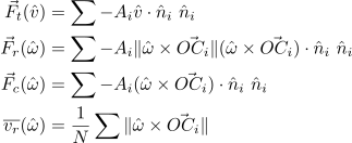
Moment of these forces relative to the point
can be obtained in a similar way. And as a result, we get the following:
Where:
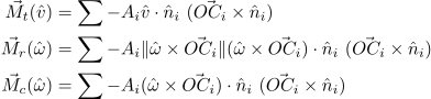
Given the above definitions, we can now form a vector
: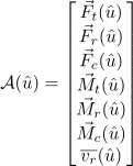
This is a vector of 19 values and we refer to the sample table
, but we can find fairly close values, and then either use them directly, or use them to interpolate the output. And at this stage, the cubic map described in the article comes into play.Appendix 2: center of mass
You may notice that the values shown above are calculated relative to an arbitrary point
. The total force acting on the body is simply the sum of all the forces:
Moments
are set as:
and the total moment of these forces relative to the point
is equal to:
Now it’s just a mathematical definition, a formula that cannot be used directly to change the movement of the body, because the center of gravity
in this formula, according to the Schall theorem, is equal to:
We recognize the moment of forces with respect to
, so: 
And it is very useful for us if we calculated the total strength
unchanged and applied the following torque to the center of mass: 
At first, I decided to just take the origin of the body as a point
in the center of the bounding parallelogram of the body, which should still be close to the center of mass and localized wind sampling in the most logical place relative to the body.Appendix 3: Scaling
Another flaw appeared when balloons were introduced into the game. These balls are spherical bodies, the size of which can vary with a factor of 5 or 10. As in the case of the center of mass, it was too costly to recalculate the aerodynamic properties at run time. Is it possible to derive an analytical formula?
Figure 15 Body
Consider the body again
but now for a scaled object. We get:
Using the same approximations as the first time, and replacing
, we get: 
For the center of mass of the scaled body
.Appendix 4: Simplified Resistance Model for Parallelogram
There are many ways to approximate forces and torques for a parallelogram, and different formulas can be obtained. Compact enough, easy to implement in code and calculations at runtime, it can be inferred by ignoring the effect of angular motion on linear force and the effect of linear speed on torque. Taking bounding parallelogram size
, we can come to the following compact formulas: 

Appendix 5: Tornado Center Spline
The tornado is centered around a central curve whose shape is slowly changing. We implemented this using two consecutive Bezier cubic splines:
for the bottom and for the top. Spline has control points , , and , a controlled by points , , and . The position of the tornado itself is at a point on the ground and the highest point It starts right above the level of the cloud layer, but is late in time, slowly following the position on the earth. Since the curves are connected at one end, and coincide in space. We also used 3 horizontal reference orbits for points, and . Finally, was located exactly at the midpoints between and , a at the midpoint between and .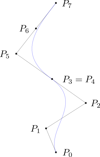 |  |
| Creating a tornado center spline | Tornado center spline evolution in time |