Kaggle: can't walk - let's run
How complex is the topic of machine learning? If you are good at mathematics, but the amount of knowledge about machine learning tends to zero, how far can you go in a serious competition on the Kaggle platform ?

Kaggle is a community of people interested in ML (from beginners to cool pros) and a venue for competitions (often with an impressive prize pool).
To immediately plunge into all the charms of ML, I decided to immediately choose a serious competition. Such was just available: Two Sigma: Using News to Predict Stock Movements . The essence of the contest in a nutshell is to predict the price of shares of various companies based on the status of the asset and news related to this asset. The prize fund of the contest is $ 100,000, which will be distributed among the participants who won the first 7 places.
The competition is special for two reasons:
By condition, we must predict confidence![$\hat{y}_{ti} \in [-1,1]$](https://habrastorage.org/getpro/habr/formulas/408/faa/39e/408faa39e905758341448a5f1dfb3560.svg) in that the return on the asset will increase. The return on an asset is considered relative to the return on the market as a whole. The target metric is custom - it is not the more familiar RMSE or MAE , but the Sharpe ratio , which in this case is considered as follows:
in that the return on the asset will increase. The return on an asset is considered relative to the return on the market as a whole. The target metric is custom - it is not the more familiar RMSE or MAE , but the Sharpe ratio , which in this case is considered as follows:
 ,
,
 - the return on asset i relative to the market for day t on a 10-day horizon,
 - a Boolean variable indicating whether the ith asset is included in the valuation for day t,
 - mean
  ,
,
 - standard deviation
  .
.
The Sharpe ratio is the risk-adjusted return, the values of the coefficient show the effectiveness of the trader:
The task is essentially the task of binary classification, that is, we predict a binary sign, will yield increase (1 class) or decrease (0 class).
Kaggle Kernels is a cloud computing platform that supports collaboration. The following types of kernels are supported:
Each kernel runs in its docker container. A large number of packages are installed in the container, a list for python can be found here . Technical specifications are as follows:
GPUs are also available in Kernels, however, GPU was prohibited in this contest.
Keras is a high-level neural network framework that runs on top of TensorFlow , CNTK, or Theano . It’s a very convenient and understandable API, and it is possible to add your network topologies, loss functions, and more using the backend API.
Scikit-learn is a large library of machine learning algorithms. A useful source of data preprocessing and data analysis algorithms for use with more specialized frameworks.
Before submitting a model for evaluation, you need to somehow check locally how well it works - that is, come up with a way to local validation. I tried the following approaches:
As a result, the results closest to the competitive assessment, oddly enough, showed a combination of the proportional partition (empirically selected the partition 0.85 / 0.15) and AUC. Cross validation is probably not very suitable, as market behavior is very different in the early stages of training data and in the evaluation period. Why the AUC worked better than the Sharpe ratio - I can not say at all.
Since the task is to predict the time series, the first to test the classical solution is a recurrent neural network ( RNN ), or rather, its variants LSTM and GRU .
The main principle of recurrent networks is that for each output value, not one sample is input, but a whole sequence. It follows that:
I generated sequences for each day, starting with t, so for fairly large t (from 20) the full set of training samples ceased to fit in memory. The problem was solved using generators, since Keras can use generators as input and output data sets for both training and prediction.
Initial preparation of the data was as naive as possible: we take the whole market data plus add a couple of features (day of the week, month, week number of the year), and we do not touch the news data at all.
The first model used t = 10 and looked like this:
Nothing adequate was squeezed out of this model, the score was near zero (even a little minus).
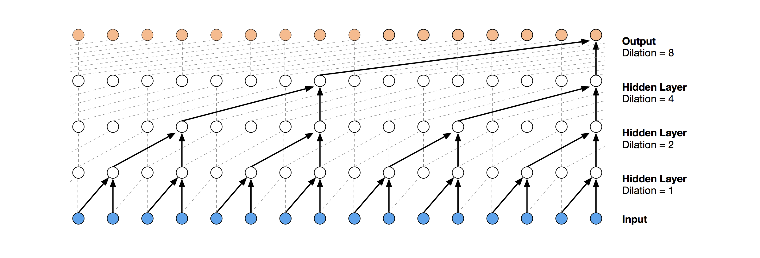
A more modern neural network solution for time series prediction is TCN. The essence of this topology is very simple: we take a one-dimensional convolutional network and apply it to our sequence of length t. More advanced options use several convolutional layers with different dilation. The TCN implementation was partially copied (sometimes at the idea level) from here (TCN stack visualization taken from the Wavenet article ).
The first relatively successful solution was this model, which includes a GRU layer on top of TCN:
Such a model produces score = 0.27668. With a little tuning (number of TCN filters, batch size) and an increase in t to 100, we get already 0.41092:
Next we add normalization and dropout:
Applying this model, including in the early steps (with t = 1), we get score = 0.53578.
At this stage, the ideas ended, and I decided to do what needed to be done at the very beginning: to see the public decisions of other participants. Most good solutions did not use neural networks at all, preferring GBM.
Gradient Boosting is an ML method, at the output of which we get an ensemble of simple models (most often decision trees). Due to the large number of such simple models, the loss function is optimized. You can read more about Gradient Boosting, for example, here .
As the implementation of GBM used lightgbm - a fairly well-known framework from Microsoft.
The model and data preprocessing taken from here immediately give a score of about 0.64:
The pre-processing here already includes news data, combining them with market data (however, doing it rather naively, only one asset code from all that are mentioned in the news is taken into account). I took this pre-processing option as the basis for all subsequent decisions.
By adding a little feature (firstMentionSentence, marketCommentary, sentimentClass), and also replacing the metric with ROC AUC , we get a score of 0.65389.
The next successful decision was to use an ensemble consisting of a neural network model and GBM (although “ensemble” is a big name for two models). The resulting prediction is obtained by averaging the predictions of the two models, thus applying the soft voting mechanism. This decision allowed to get score 0.66879.
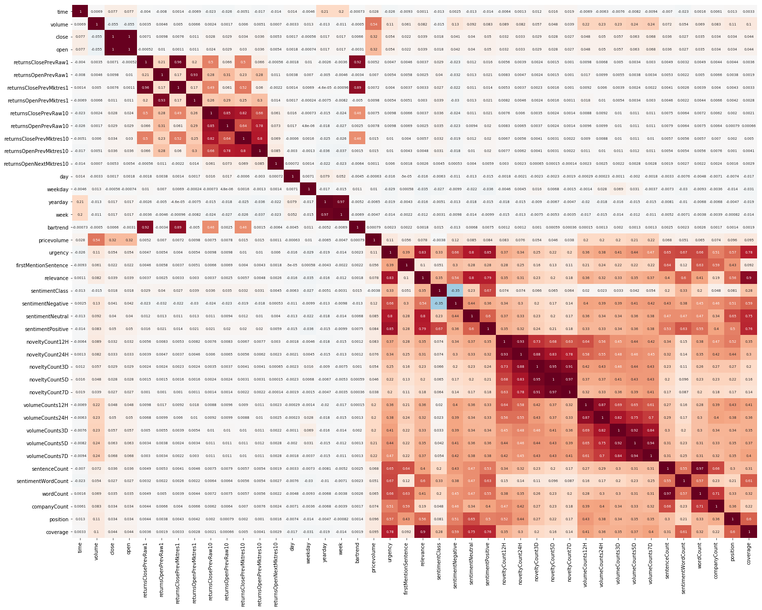
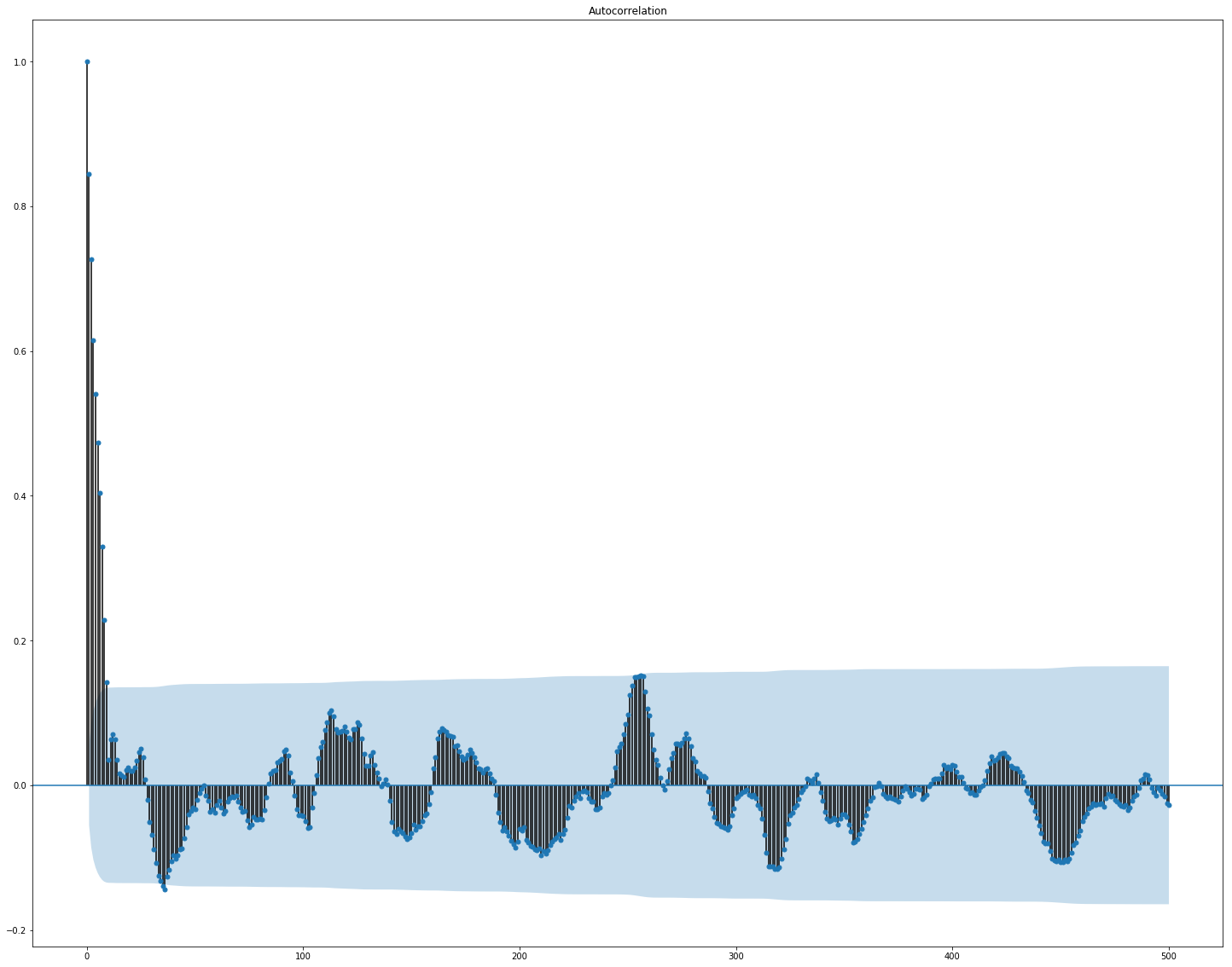
Another thing to start with was EDA. Having read that it is important to understand the correlation between features, we build such a picture (the pictures in this section are clickable): Here it is clearly visible that the correlation separately inside the market and news data is quite high, however, only the profitability values somehow correlate with the target value. Since the data represent a time series, it makes sense to also look at the autocorrelation of the target value: It can be seen that, after a 10-day period, the dependence drops significantly. This is probably what causes GBM to work well, taking into account only features with a 10-day delay (which are already in the original data set). Feature selection and preprocessing is crucial for all ML algorithms. Let's try to use automatic ways to extract features, namely
principal component analysis ( PCA ):
Let's see what features the PCA generates: We see that the method does not work very well on our data, since the final correlation of new features with the target value is small.

Many ML models have a fairly large number of hyperparameters, that is, the “settings” of the algorithm itself. They can be selected manually, but there are also automatic selection mechanisms. For the latter, there is a hyperopt library that implements two matching algorithms - random search and Tree-structured Parzen Estimator (TPE) . I tried to optimize:
As a result, all the solutions found using this optimization gave a lower score, although they worked better on the test data. Probably, the reason lies in the fact that the data for which the score is considered are not very similar to the validation data selected from the training. Thus, for this task, fine tuning is not very suitable, as it leads to retraining of the model.
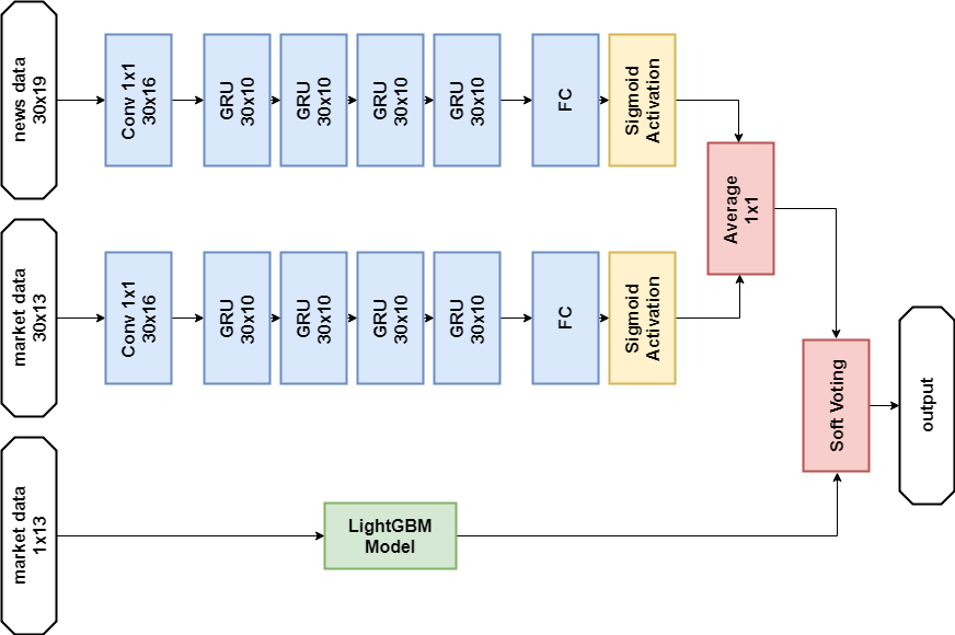
According to the rules of the competition, participants can choose two solutions for the final stage. My final decisions are almost the same and contain an ensemble of two models - GBM and multilayer GRU . The only difference is that one solution does not use news data at all, and the other one uses it, but only for the neural network model.
News Data Solution:
Solution without news data:

Both decisions yielded a similar result (about 0.69) at the first stage of the competition, which corresponded to 566 out of 2,927 places. After the first month of new data, the positions in the list of participants mixed up strongly, and the solution with news data was in 65th place from the remaining 697 teams with the result of 3.19251, and what will happen over the next five months, no one knows.
Since decisions are evaluated using the Sharpe ratio, it is logical to try to use it as a metric for early termination of training.
Metric for lightgbm:
Verification showed that such a metric works worse in this problem than AUC.
The attention mechanism allows the neural network to focus on the “most important” features in the source data. Technically, attention is represented by a vector of weights (most often obtained using a fully connected layer with softmax activation ), which are multiplied by the output of another layer. I used an implementation in which attention is applied to the time axis:
This model looks pretty pretty, but this approach did not give a score increase, it turned out to be about 0.67.
Several areas that look promising:
Our adventure has come to an end, you can try to summarize. The competition turned out to be difficult, but we could not face the dirt. This hints that the threshold for entering the ML is not so high, but, as in any business, real magic (and there is plenty of it in machine learning) is already available to professionals.
Results in numbers:
Обращаю внимание, что цифры по второму этапу пока ни о чем особенно не говорят, так как данных пока еще очень мало для качественной оценки решений.
Финальное решение с использованием новостей
Two Sigma: Using News to Predict Stock Movements — страница конкурса
Keras — нейросетевой фреймворк
LightGBM — GBM фреймворк
Scikit-learn — библиотека алгоритмов машинного обучения
Hyperopt — библиотека для оптимизации гиперпараметров
Статья о WaveNet

About the site and the competition
Kaggle is a community of people interested in ML (from beginners to cool pros) and a venue for competitions (often with an impressive prize pool).
To immediately plunge into all the charms of ML, I decided to immediately choose a serious competition. Such was just available: Two Sigma: Using News to Predict Stock Movements . The essence of the contest in a nutshell is to predict the price of shares of various companies based on the status of the asset and news related to this asset. The prize fund of the contest is $ 100,000, which will be distributed among the participants who won the first 7 places.
The competition is special for two reasons:
- this is a Kernels-only contest: you can train models only in the Kaggle Kernels cloud;
- the final distribution of seats will be known only six months after the completion of decision-making; during this time, decisions will predict prices at the current date.
About the task
By condition, we must predict confidence
The Sharpe ratio is the risk-adjusted return, the values of the coefficient show the effectiveness of the trader:
- less than 1: poor performance
- 1 - 2: medium, normal efficiency,
- 2 - 3: excellent performance,
- over 3: perfect.
Market Movement Data
- time (datetime64 [ns, UTC]) - current time (in the data on market movement in all lines at 22:00 UTC)
- assetCode (object) - asset identifier
- assetName (category) - an identifier of an asset group for communication with news data
- universe (float64) - a boolean value indicating whether this asset will be taken into account in the calculation of score
- volume (float64) - daily trading volume
- close (float64) - closing price for this day
- open (float64) - open price for this day
- returnsClosePrevRaw1 (float64) - yield from closing to closing for the previous day
- returnsOpenPrevRaw1 (float64) - profitability from opening to opening for the previous day
- returnsClosePrevMktres1 (float64) - profitability from closing to closing for the previous day, adjusted relative to the movement of the market as a whole
- returnsOpenPrevMktres1 (float64) - profitability from opening to opening for the previous day, adjusted relative to the movement of the market as a whole
- returnsClosePrevRaw10 (float64) - yield from close to close for the previous 10 days
- returnsOpenPrevRaw10 (float64) - profitability from opening to opening for the previous 10 days
- returnsClosePrevMktres10 (float64) - yield from close to close for the previous 10 days, adjusted relative to the movement of the market as a whole
- returnsOpenPrevMktres10 (float64) - yield from opening to opening for the previous 10 days, adjusted relative to the movement of the market as a whole
- returnsOpenNextMktres10 (float64) - yield from open to open over the next 10 days, adjusted for the movement of the market as a whole. We will predict this value.
News data
- time (datetime64 [ns, UTC]) - time in UTC data availability
- sourceTimestamp (datetime64 [ns, UTC]) - time in UTC publication news
- firstCreated (datetime64 [ns, UTC]) - time in UTC of the first version of the data
- sourceId (object) - record identifier
- headline (object) - header
- urgency (int8) - types of news (1: alert, 3: article)
- takeSequence (int16) - not quite clear parameter, number in some sequence
- provider (category) - news provider identifier
- subjects (category) - a list of news topic codes (may be a geographical sign, event, industry sector, etc.)
- audiences (category) - list of audience codes news
- bodySize (int32) - number of characters in the news body
- companyCount (int8) - number of companies explicitly mentioned in the news
- headlineTag (object) - a certain title tag from Thomson Reuters
- marketCommentary (bool) - a sign that the news relates to general market conditions
- sentenceCount (int16) - number of offers in the news
- wordCount (int32) - number of words and punctuation marks in the news
- assetCodes (category) - list of assets mentioned in the news
- assetName (category) - asset group code
- firstMentionSentence (int16) - a sentence that first mentions an asset:
- relevance (float32) - a number from 0 to 1, showing the relevance of the news regarding the asset
- sentimentClass (int8) - news tonality class
- sentimentNegative (float32) - probability that tonality is negative
- sentimentNeutral (float32) - probability that the tone is neutral
- sentimentPositive (float32) - probability that the key is positive
- sentimentWordCount (int32) - the number of words in the text that are related to the asset
- noveltyCount12H (int16) - “novelty” news in 12 hours, calculated relative to previous news about this asset
- noveltyCount24H (int16) - same, in 24 hours
- noveltyCount3D (int16) - same, in 3 days
- noveltyCount5D (int16) - same, in 5 days
- noveltyCount7D (int16) - same, in 7 days
- volumeCounts12H (int16) - the amount of news about this asset in 12 hours
- volumeCounts24H (int16) - same, in 24 hours
- volumeCounts3D (int16) - same, in 3 days
- volumeCounts5D (int16) - same, for 5 days
- volumeCounts7D (int16) - same, in 7 days
The task is essentially the task of binary classification, that is, we predict a binary sign, will yield increase (1 class) or decrease (0 class).
About Tools
Kaggle Kernels is a cloud computing platform that supports collaboration. The following types of kernels are supported:
- Python script
- R script
- Jupyter notebook
- RMarkdown
Each kernel runs in its docker container. A large number of packages are installed in the container, a list for python can be found here . Technical specifications are as follows:
- CPU: 4 cores,
- RAM: 17 GB,
- drive: 5 GB permanent and 16 GB temporary,
- maximum script run time: 9 hours (at the time of the start of the competition it was 6 hours).
GPUs are also available in Kernels, however, GPU was prohibited in this contest.
Keras is a high-level neural network framework that runs on top of TensorFlow , CNTK, or Theano . It’s a very convenient and understandable API, and it is possible to add your network topologies, loss functions, and more using the backend API.
Scikit-learn is a large library of machine learning algorithms. A useful source of data preprocessing and data analysis algorithms for use with more specialized frameworks.
Model validation
Before submitting a model for evaluation, you need to somehow check locally how well it works - that is, come up with a way to local validation. I tried the following approaches:
- cross validation vs simple proportional division into training / test sets;
- local calculation of the Sharpe ratio vs ROC AUC .
As a result, the results closest to the competitive assessment, oddly enough, showed a combination of the proportional partition (empirically selected the partition 0.85 / 0.15) and AUC. Cross validation is probably not very suitable, as market behavior is very different in the early stages of training data and in the evaluation period. Why the AUC worked better than the Sharpe ratio - I can not say at all.
First attempts
Since the task is to predict the time series, the first to test the classical solution is a recurrent neural network ( RNN ), or rather, its variants LSTM and GRU .
The main principle of recurrent networks is that for each output value, not one sample is input, but a whole sequence. It follows that:
- we need some preprocessing of the initial data — the generation of these very sequences of length t days for each asset;
- a model based on a recurrent network cannot predict the output value if there is no data for the previous t days.
I generated sequences for each day, starting with t, so for fairly large t (from 20) the full set of training samples ceased to fit in memory. The problem was solved using generators, since Keras can use generators as input and output data sets for both training and prediction.
Initial preparation of the data was as naive as possible: we take the whole market data plus add a couple of features (day of the week, month, week number of the year), and we do not touch the news data at all.
The first model used t = 10 and looked like this:
model = Sequential()
model.add(LSTM(256, activation=act.tanh, return_sequences=True, input_shape=(data.timesteps, data.features)))
model.add(LSTM(256, activation=act.relu))
model.add(Dense(data.assets, activation=act.relu))
model.add(Dense(data.assets))
Nothing adequate was squeezed out of this model, the score was near zero (even a little minus).
Temporal Convolutional Networks
A more modern neural network solution for time series prediction is TCN. The essence of this topology is very simple: we take a one-dimensional convolutional network and apply it to our sequence of length t. More advanced options use several convolutional layers with different dilation. The TCN implementation was partially copied (sometimes at the idea level) from here (TCN stack visualization taken from the Wavenet article ).

The first relatively successful solution was this model, which includes a GRU layer on top of TCN:
model = Sequential()
model.add(Conv1D(512,3, activation=act.relu, padding='causal', input_shape=(data.timesteps, data.features)))
model.add(Conv1D(100,3, activation=act.relu, padding='causal', dilation_rate=2))
model.add(Conv1D(100,3, activation=act.relu, padding='causal', dilation_rate=4))
model.add(GRU(256))
model.add(Dense(data.assets, activation=act.relu))
Such a model produces score = 0.27668. With a little tuning (number of TCN filters, batch size) and an increase in t to 100, we get already 0.41092:
batch_size = 512
model = Sequential()
model.add(Conv1D(8,3, activation=act.relu, padding='causal', input_shape=(data.timesteps, data.features)))
model.add(Conv1D(4,3, activation=act.relu, padding='causal', dilation_rate=2))
model.add(Conv1D(4,3, activation=act.relu, padding='causal', dilation_rate=4))
model.add(GRU(16))
model.add(Dense(1, activation=act.sigmoid))
Next we add normalization and dropout:
The code
batch_size = 512
dropout_rate = 0.05
def channel_normalization(x):
	max_values = K.max(K.abs(x), 2, keepdims=True) + 1e-5
	out = x / max_values
	return out
model = Sequential()
if(data.timesteps > 1):
	model.add(Conv1D(16,2, activation=act.relu, padding='valid', input_shape=(data.timesteps, data.features)))
	model.add(Lambda(channel_normalization))
	model.add(SpatialDropout1D(dropout_rate))
	model.add(Conv1D(16,1, padding='valid'))
	for i in range(1, 6):
		model.add(Conv1D(16,2, activation=act.relu, padding='valid', dilation_rate=2**i))
		model.add(Lambda(channel_normalization))
		model.add(SpatialDropout1D(dropout_rate))
		model.add(Conv1D(16,1, padding='valid'))
	model.add(Flatten())
else:
	model.add(Flatten(input_shape=(data.timesteps, data.features)))
	model.add(Dense(256, activation=act.relu))
model.add(Dense(1, activation=act.sigmoid))
Applying this model, including in the early steps (with t = 1), we get score = 0.53578.
Gradient Boosting Machines
At this stage, the ideas ended, and I decided to do what needed to be done at the very beginning: to see the public decisions of other participants. Most good solutions did not use neural networks at all, preferring GBM.
Gradient Boosting is an ML method, at the output of which we get an ensemble of simple models (most often decision trees). Due to the large number of such simple models, the loss function is optimized. You can read more about Gradient Boosting, for example, here .
As the implementation of GBM used lightgbm - a fairly well-known framework from Microsoft.
The model and data preprocessing taken from here immediately give a score of about 0.64:
The code
def prepare_data(marketdf, newsdf):
	# a bit of feature engineering
	marketdf['time'] = marketdf.time.dt.strftime("%Y%m%d").astype(int)
	marketdf['bartrend'] = marketdf['close'] / marketdf['open']
	marketdf['average'] = (marketdf['close'] + marketdf['open'])/2
	marketdf['pricevolume'] = marketdf['volume'] * marketdf['close']
	newsdf['time'] = newsdf.time.dt.strftime("%Y%m%d").astype(int)
	newsdf['assetCode'] = newsdf['assetCodes'].map(lambda x: list(eval(x))[0])
	newsdf['position'] = newsdf['firstMentionSentence'] / newsdf['sentenceCount']
	newsdf['coverage'] = newsdf['sentimentWordCount'] / newsdf['wordCount']
	# filter pre-2012 data, no particular reason
	marketdf = marketdf.loc[marketdf['time'] > 20120000]
	# get rid of extra junk from news data
	droplist = ['sourceTimestamp','firstCreated','sourceId','headline','takeSequence','provider','firstMentionSentence', 'sentenceCount','bodySize','headlineTag','marketCommentary','subjects','audiences','sentimentClass', 'assetName', 'assetCodes','urgency','wordCount','sentimentWordCount']
	newsdf.drop(droplist, axis=1, inplace=True)
	marketdf.drop(['assetName', 'volume'], axis=1, inplace=True)
	# combine multiple news reports for same assets on same day
	newsgp = newsdf.groupby(['time','assetCode'], sort=False).aggregate(np.mean).reset_index()
	# join news reports to market data, note many assets will have many days without news data
	return pd.merge(marketdf, newsgp, how='left', on=['time', 'assetCode'], copy=False)
import lightgbm as lgb
print ('Training lightgbm')
# money
params = {
	"objective" : "binary",
	"metric" : "binary_logloss",
	"num_leaves" : 60,
	"max_depth": -1,
	"learning_rate" : 0.01,
	"bagging_fraction" : 0.9, # subsample
	"feature_fraction" : 0.9, # colsample_bytree
	"bagging_freq" : 5, # subsample_freq
	"bagging_seed" : 2018,
	"verbosity" : -1
}
lgtrain, lgval = lgb.Dataset(Xt, Yt[:,0]), lgb.Dataset(Xv, Yv[:,0])
lgbmodel = lgb.train(params, lgtrain, 2000, valid_sets=[lgtrain, lgval], early_stopping_rounds=100, verbose_eval=200)
The pre-processing here already includes news data, combining them with market data (however, doing it rather naively, only one asset code from all that are mentioned in the news is taken into account). I took this pre-processing option as the basis for all subsequent decisions.
By adding a little feature (firstMentionSentence, marketCommentary, sentimentClass), and also replacing the metric with ROC AUC , we get a score of 0.65389.
Ensemble
The next successful decision was to use an ensemble consisting of a neural network model and GBM (although “ensemble” is a big name for two models). The resulting prediction is obtained by averaging the predictions of the two models, thus applying the soft voting mechanism. This decision allowed to get score 0.66879.
Exploratory Data Analysis and Feature Engineering
Another thing to start with was EDA. Having read that it is important to understand the correlation between features, we build such a picture (the pictures in this section are clickable): Here it is clearly visible that the correlation separately inside the market and news data is quite high, however, only the profitability values somehow correlate with the target value. Since the data represent a time series, it makes sense to also look at the autocorrelation of the target value: It can be seen that, after a 10-day period, the dependence drops significantly. This is probably what causes GBM to work well, taking into account only features with a 10-day delay (which are already in the original data set). Feature selection and preprocessing is crucial for all ML algorithms. Let's try to use automatic ways to extract features, namely


principal component analysis ( PCA ):
from sklearn.decomposition import PCA
from sklearn.preprocessing import StandardScaler
market_x = market_data.loc[:,features]
scaler = StandardScaler()
scaler.fit(market_x)
market_x = scaler.transform(market_x)
pca = PCA(.95)
pca.fit(market_x)
market_pca = pca.transform(market_x)
Let's see what features the PCA generates: We see that the method does not work very well on our data, since the final correlation of new features with the target value is small.

Fine tuning and whether it is needed
Many ML models have a fairly large number of hyperparameters, that is, the “settings” of the algorithm itself. They can be selected manually, but there are also automatic selection mechanisms. For the latter, there is a hyperopt library that implements two matching algorithms - random search and Tree-structured Parzen Estimator (TPE) . I tried to optimize:
- lightgbm parameters (type of algorithm, number of leaves, learning rate and others),
- parameters of neural network models (number of TCN filters , number of GRU memory blocks , dropout rate, learning rate, solver type).
As a result, all the solutions found using this optimization gave a lower score, although they worked better on the test data. Probably, the reason lies in the fact that the data for which the score is considered are not very similar to the validation data selected from the training. Thus, for this task, fine tuning is not very suitable, as it leads to retraining of the model.
Final decision
According to the rules of the competition, participants can choose two solutions for the final stage. My final decisions are almost the same and contain an ensemble of two models - GBM and multilayer GRU . The only difference is that one solution does not use news data at all, and the other one uses it, but only for the neural network model.
News Data Solution:

Imports
import numpy as np
import pandas as p
import itertools
import functools
from kaggle.competitions import twosigmanews
from sklearn.preprocessing import StandardScaler, LabelEncoder
import tensorflow as tf
from keras.models import Sequential, Model
from keras.layers import Dense, GRU, LSTM, Conv1D, Reshape, Flatten, SpatialDropout1D, Lambda, Input, Average
from keras.optimizers import Adam, SGD, RMSprop
from keras import losses as ls
from keras import activations as act
import keras.backend as K
import lightgbm as lgb
Data preprocessing
# fix random
from numpy.random import seed
seed(42)
from tensorflow import set_random_seed
set_random_seed(42)
env = twosigmanews.make_env()
(market_train_df, news_train_df) = env.get_training_data()
def cleanData(market_data, news_data):
    market_data = market_data[(market_data['returnsOpenNextMktres10'] <= 1) & (market_data['returnsOpenNextMktres10'] >= -1)]
    return market_data, news_data
def prepareData(marketdf, newsdf, scaler=None):
    print('Preparing data...')
    print('...preparing features...')
    marketdf = marketdf.copy()
    newsdf = newsdf.copy()
    # a bit of feature engineering
    marketdf['time'] = marketdf.time.dt.strftime("%Y%m%d").astype(int)
    marketdf['bartrend'] = marketdf['close'] / marketdf['open']
    marketdf['average'] = (marketdf['close'] + marketdf['open'])/2
    marketdf['pricevolume'] = marketdf['volume'] * marketdf['close']
    newsdf['time'] = newsdf.time.dt.strftime("%Y%m%d").astype(int)
    newsdf['position'] = newsdf['firstMentionSentence'] / newsdf['sentenceCount']
    newsdf['coverage'] = newsdf['sentimentWordCount'] / newsdf['wordCount']
    # filter pre-2012 data, no particular reason
    marketdf = marketdf.loc[marketdf['time'] > 20120000]
    # get rid of extra junk from news data
    droplist = ['sourceTimestamp','firstCreated','sourceId','headline','takeSequence','provider',
                'sentenceCount','bodySize','headlineTag', 'subjects','audiences',
                'assetName', 'wordCount','sentimentWordCount', 'companyCount',
                 'coverage']
    newsdf.drop(droplist, axis=1, inplace=True)
    marketdf.drop(['assetName', 'volume'], axis=1, inplace=True)
    # unstack news
    newsdf['assetCodes'] = newsdf['assetCodes'].apply(lambda x: x[1:-1].replace("'", ""))
    codes = []
    indices = []
    for i, values in newsdf['assetCodes'].iteritems():
        explode = values.split(", ")
        codes.extend(explode)
        repeat_index = [int(i)]*len(explode)
        indices.extend(repeat_index)
    index_df = p.DataFrame({'news_index': indices, 'assetCode': codes})
    newsdf['news_index'] = newsdf.index.copy()
    # Merge news on unstacked assets
    news_unstack = index_df.merge(newsdf, how='left', on='news_index')
    news_unstack.drop(['news_index', 'assetCodes'], axis=1, inplace=True)
    # combine multiple news reports for same assets on same day
    newsgp = news_unstack.groupby(['time','assetCode'], sort=False).aggregate(np.mean).reset_index()
    # join news reports to market data, note many assets will have many days without news data
    res = p.merge(marketdf, newsgp, how='left', on=['time', 'assetCode'], copy=False) #, right_on=['time', 'assetCodes'])
    res.marketCommentary = res.marketCommentary.astype(float)
    targetcol = 'returnsOpenNextMktres10'
    target_presented = targetcol in res.columns
    features = [col for col in res.columns if col not in ['time', 'assetCode', 'universe', targetcol]]
    print('...scaling...')
    if(scaler == None):
        scaler = StandardScaler()
        scaler = scaler.fit(res[features])
    res[features] = scaler.transform(res[features])
    print('...done.')
    return type('', (object,), {
        'scaler': scaler,
        'data': res,
        'x': res[features],
        'y': (res[targetcol] > 0).astype(int).values if target_presented else None,
        'features': features,
        'samples': len(res),
        'assets': res['assetCode'].unique(),
        'target_presented': target_presented
    })
def generateTimeSeries(data, n_timesteps=1):
    data.data[data.features] = data.data[data.features].fillna(data.data[data.features].mean())
    #data.data[data.features] = data.data[data.features].fillna(0)
    assets = data.data.groupby('assetCode', sort=False)
    def grouper(n, iterable):
        it = iter(iterable)
        while True:
           chunk = list(itertools.islice(it, n))
           if not chunk:
               return
           yield chunk
    def sample_generator():
        while True:
            for assetCode, days in assets:
                x = days[data.features].values
                y = (days['returnsOpenNextMktres10'] > 0).astype(int).values if data.target_presented else None
                for i in range(0, len(days) - n_timesteps + 1):
                    yield (x[i: i + n_timesteps], y[i + n_timesteps - 1] if data.target_presented else 0)
    def batch_generator(batch_size):
        for batch in grouper(batch_size, sample_generator()):
            yield tuple([np.array(t) for t in zip(*batch)])
    n_samples = functools.reduce(lambda x,y : x + y, map(lambda t : 0 if len(t[1]) + 1 <= n_timesteps else len(t[1]) - n_timesteps + 1, assets))
    return type('', (object,), {
        'gen': batch_generator,
        'timesteps': n_timesteps,
        'features': len(data.features),
        'samples': n_samples,
        'assets': list(map(lambda x: x[0], filter(lambda t : len(t[1]) + 1 > n_timesteps, assets)))
    })
Neural network model
def buildRNN(timesteps, features):
    i = Input(shape=(timesteps, features))
    x1 = Lambda(lambda x: x[:,:,:13])(i)
    x1 = Conv1D(16,1, padding='valid')(x1)
    x1 = GRU(10, return_sequences=True)(x1)
    x1 = GRU(10, return_sequences=True)(x1)
    x1 = GRU(10, return_sequences=True)(x1)
    x1 = GRU(10)(x1)
    x1 = Dense(1, activation=act.sigmoid)(x1)
    x2 = Lambda(lambda x: x[:,:,13:])(i)
    x2 = Conv1D(16,1, padding='valid')(x2)
    x2 = GRU(10, return_sequences=True)(x2)
    x2 = GRU(10, return_sequences=True)(x2)
    x2 = GRU(10, return_sequences=True)(x2)
    x2 = GRU(10)(x2)
    x2 = Dense(1, activation=act.sigmoid)(x2)
    x = Average()([x1, x2])
    model = Model(inputs=i, outputs=x)
    return model
def train_model_time_series(model, data, val_data=None):
    print('Building model...')
    batch_size = 4096
    optimizer = RMSprop()
    # define roc_callback, inspired by https://github.com/keras-team/keras/issues/6050#issuecomment-329996505
    def auc_roc(y_true, y_pred):
        value, update_op = tf.metrics.auc(y_true, y_pred)
        metric_vars = [i for i in tf.local_variables() if 'auc_roc' in i.name.split('/')[1]]
        for v in metric_vars:
            tf.add_to_collection(tf.GraphKeys.GLOBAL_VARIABLES, v)
        with tf.control_dependencies([update_op]):
            value = tf.identity(value)
            return value
    model.compile(loss=ls.binary_crossentropy, optimizer=optimizer, metrics=['binary_accuracy', auc_roc])
    print(model.summary())
    print('Training model...')
    if(val_data == None):
        model.fit_generator(data.gen(batch_size),
            epochs=8,
            steps_per_epoch=int(data.samples / batch_size),
            verbose=1)
    else:
        model.fit_generator(data.gen(batch_size),
            epochs=8,
            steps_per_epoch=int(data.samples / batch_size),
            validation_data=val_data.gen(batch_size),
            validation_steps=int(val_data.samples / batch_size),
            verbose=1)
    return type('', (object,), {
        'predict': lambda x: model.predict_generator(x, steps=1)
    })
GBM model
def train_model(data, val_data=None):
    print('Building model...')
    params = {
        "objective" : "binary",
        "metric" : "auc",
        "num_leaves" : 60,
        "max_depth": -1,
        "learning_rate" : 0.01,
        "bagging_fraction" : 0.9,  # subsample
        "feature_fraction" : 0.9,  # colsample_bytree
        "bagging_freq" : 5,        # subsample_freq
        "bagging_seed" : 2018,
        "verbosity" : -1 }
    ds, val_ds = lgb.Dataset(data.x.iloc[:,:13], data.y), lgb.Dataset(val_data.x.iloc[:,:13], val_data.y)
    print('...training...')
    model = lgb.train(params, ds, 2000, valid_sets=[ds, val_ds], early_stopping_rounds=100, verbose_eval=100)
    print('...done.')
    return type('', (object,), {
        'model': model,
        'predict': lambda x: model.predict(x.iloc[:,:13], num_iteration=model.best_iteration)
    })
Training
n_timesteps = 30
market_data, news_data = cleanData(market_train_df, news_train_df)
dates = market_data['time'].unique()
train = range(len(dates))[:int(0.85*len(dates))]
val = range(len(dates))[int(0.85*len(dates)):]
train_data_prepared = prepareData(market_data.loc[market_data['time'].isin(dates[train])], news_data.loc[news_data['time'] <= max(dates[train])])
val_data_prepared = prepareData(market_data.loc[market_data['time'].isin(dates[val])], news_data.loc[news_data['time'] > max(dates[train])], scaler=train_data_prepared.scaler)
model_gbm = train_model(train_data_prepared, val_data_prepared)
train_data_ts = generateTimeSeries(train_data_prepared, n_timesteps=n_timesteps)
val_data_ts = generateTimeSeries(val_data_prepared, n_timesteps=n_timesteps)
rnn = buildRNN(train_data_ts.timesteps, train_data_ts.features)
model_rnn = train_model_time_series(rnn, train_data_ts, val_data_ts)
Prediction
def make_predictions(data, template, model):
    if(hasattr(data, 'gen')):
        prediction = (model.predict(data.gen(data.samples)) * 2 - 1)[:,-1]
    else:
        prediction = model.predict(data.x) * 2 - 1
    predsdf = p.DataFrame({'ast':data.assets,'conf':prediction})
    template['confidenceValue'][template['assetCode'].isin(predsdf.ast)] = predsdf['conf'].values
    return template
day = 1
days_data = p.DataFrame({})
days_data_len = []
days_data_n = p.DataFrame({})
days_data_n_len = []
for (market_obs_df, news_obs_df, predictions_template_df) in env.get_prediction_days():
    print(f'Predicting day {day}')
    days_data = p.concat([days_data, market_obs_df], ignore_index=True, copy=False, sort=False)
    days_data_len.append(len(market_obs_df))
    days_data_n = p.concat([days_data_n, news_obs_df], ignore_index=True, copy=False, sort=False)
    days_data_n_len.append(len(news_obs_df))
    data = prepareData(market_obs_df, news_obs_df, scaler=train_data_prepared.scaler)
    predictions_df = make_predictions(data, predictions_template_df.copy(), model_gbm)
    if(day >= n_timesteps):
        data = prepareData(days_data, days_data_n, scaler=train_data_prepared.scaler)
        data = generateTimeSeries(data, n_timesteps=n_timesteps)
        predictions_df_s = make_predictions(data, predictions_template_df.copy(), model_rnn)
        predictions_df['confidenceValue'] = (predictions_df['confidenceValue'] + predictions_df_s['confidenceValue']) / 2
        days_data = days_data[days_data_len[0]:]
        days_data_n = days_data_n[days_data_n_len[0]:]
        days_data_len = days_data_len[1:]
        days_data_n_len = days_data_n_len[1:]
    env.predict(predictions_df)
    day += 1
env.write_submission_file()
Solution without news data:

Code (only a different method)
def buildRNN(timesteps, features):
    i = Input(shape=(timesteps, features))
    x1 = Lambda(lambda x: x[:,:,:13])(i)
    x1 = Conv1D(16,1, padding='valid')(x1)
    x1 = GRU(10, return_sequences=True)(x1)
    x1 = GRU(10, return_sequences=True)(x1)
    x1 = GRU(10, return_sequences=True)(x1)
    x1 = GRU(10)(x1)
    x1 = Dense(1, activation=act.sigmoid)(x1)
    model = Model(inputs=i, outputs=x1)
    return model
Both decisions yielded a similar result (about 0.69) at the first stage of the competition, which corresponded to 566 out of 2,927 places. After the first month of new data, the positions in the list of participants mixed up strongly, and the solution with news data was in 65th place from the remaining 697 teams with the result of 3.19251, and what will happen over the next five months, no one knows.
What else did i try
Custom metrics
Since decisions are evaluated using the Sharpe ratio, it is logical to try to use it as a metric for early termination of training.
Metric for lightgbm:
def sharpe_metric(y_pred, train_data):
	y_true = train_data.get_label() * 2 - 1
	std =  np.std(y_true * y_pred)
	mean = np.mean(y_true * y_pred)
	sharpe = np.divide(mean, std, out=np.zeros_like(mean), where=std!=0)
	return "sharpe", sharpe, True
Verification showed that such a metric works worse in this problem than AUC.
Attention mechanism
The attention mechanism allows the neural network to focus on the “most important” features in the source data. Technically, attention is represented by a vector of weights (most often obtained using a fully connected layer with softmax activation ), which are multiplied by the output of another layer. I used an implementation in which attention is applied to the time axis:
def buildRNN(timesteps, features):
    def attention_3d_block(inputs):
        a = Permute((2, 1))(inputs)
        a = Dense(timesteps, activation=act.softmax)(a)
        a = Permute((2, 1))(a)
        mul = Multiply()([inputs, a])
        return mul
    i = Input(shape=(timesteps, features))
    x1 = Lambda(lambda x: x[:,:,:13])(i)
    x1 = Conv1D(16,1, padding='valid')(x1)
    x1 = GRU(10, return_sequences=True)(x1)
    x1 = attention_3d_block(x1)
    x1 = GRU(10, return_sequences=True)(x1)
    x1 = attention_3d_block(x1)
    x1 = GRU(10, return_sequences=True)(x1)
    x1 = attention_3d_block(x1)
    x1 = GRU(10)(x1)
    x1 = Dense(1, activation=act.sigmoid)(x1)
    model = Model(inputs=i, outputs=x1)
    return model
This model looks pretty pretty, but this approach did not give a score increase, it turned out to be about 0.67.
What did not have time to do
Several areas that look promising:
- more specifically deal with the mechanism of attention ,
- try using auto encoders ,
- try online learning ,
- Carefully deal with the integration of news and market data, as well as with pre-processing news.
conclusions
Our adventure has come to an end, you can try to summarize. The competition turned out to be difficult, but we could not face the dirt. This hints that the threshold for entering the ML is not so high, but, as in any business, real magic (and there is plenty of it in machine learning) is already available to professionals.
Results in numbers:
- The maximum score in the first stage: ~ 0.69 against ~ 1.5 in the first place. Something like the average for the hospital, a value of 0.7 was overcome by a few, the maximum score of the public decision was also ~ 0.69, slightly more than mine.
- Place in the first stage: 566 out of 2927.
- Score in the second stage: 3.19251 after the first month.
- Place in the second stage: 65 out of 697 after the first month.
Обращаю внимание, что цифры по второму этапу пока ни о чем особенно не говорят, так как данных пока еще очень мало для качественной оценки решений.
Ссылки
Финальное решение с использованием новостей
Two Sigma: Using News to Predict Stock Movements — страница конкурса
Keras — нейросетевой фреймворк
LightGBM — GBM фреймворк
Scikit-learn — библиотека алгоритмов машинного обучения
Hyperopt — библиотека для оптимизации гиперпараметров
Статья о WaveNet
