How many programmers do you need to support previously written code?
Some time ago, a conversation took place between me and my good friend, in which the following phrases were heard:
- The number of programmers will constantly grow - because the amount of code is growing, and more and more developers are constantly needed to support it.
- But the code is aging, part of it is leaving support. The presence of some kind of equilibrium is not ruled out.
Recalling them a few days later, I wondered if the code support, requiring more and more resources over time, could ultimately paralyze the development of new functionality, or would require an unlimited increase in the number of programmers? Mathematical analysis and differential equations helped to qualitatively assess the dependence of the volume of support on development and find answers to questions.
Consider a team of programmers in which the number of participants is constant. Share of their working time (
( ) accounted for by the development of new code, and the remaining fraction of the time
  goes to support. Under the assumptions of the model, suppose that the first type of activity is aimed at increasing the amount of code, and the second - at changing it (correcting errors) and does not significantly affect the amount of code.
We denote all code written by time
  . Considering the speed of writing code is proportionalwe get:
It is natural to assume that the labor involved in maintaining the code is proportional to its volume:
or
Where from
We get a differential equation that integrates easily. If at the initial moment of time the amount of code is zero, then
At function
  , a
, a  . And this means a gradual reduction over time of the development of new functionality to zero and the transition of all resources to support.
However, if in time Since the code becomes obsolete and ceases to be supported, the amount of code requiring support at a time equal to
  Then
Then
a is a solution of a differential equation with a delayed argument [1]:
The solution to this equation is uniquely determined by setting the values "Before the beginning of time", with ![$ t \ in [-h, 0] $](https://habrastorage.org/getpro/habr/formulas/006/950/a6c/006950a6c5cbcf25dc729089b5161286.svg) . Since no code was written before the initial time, in our case
. Since no code was written before the initial time, in our case at .
at .
Let's look at a few examples. We will measure time in years, and the amount of code in thousands of lines. Then for Values of the order of tens are acceptable, we take 50 and 100. That is, in a year the development team will write fifty and one hundred thousand lines of code, respectively. For
 acceptable values may be:
  ,
,  ,
,  . This means that the development team is able to maintain the amount of code that it wrote for the year, with a quarter, half, or full workload. As the average life time of the code, let us set the values: 1, 2, and 4 years. Solving the equation numerically, we obtain examples of the behavior of the function for some combinations of parameters
  .
.
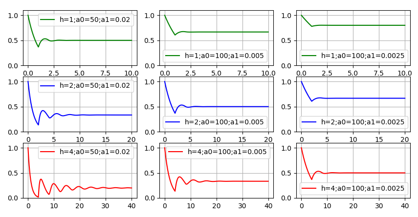
Function Behaviorin the face of aging code has changed. The function has ceased to be monotonous, but fluctuations “calm down” over time, there is a tendency towardsto some constant value. Charts show: the more , and , that is, the slower the code gets older, the faster the development of new code occurs and the lower the quality of the code, the less resources will remain for the development of new functionality. There was a desire to give at least one example in which"Snuggled" close to zero. But this required the selection of very poor development quality indicators and long-aging code. Even in the lower left graph, a significant amount of resources remains for the new functionality. Therefore, the correct answer to the first question is more likely this: theoretically - yes, it is possible; practically - hardly.
Questions that could not be answered:
We denote number of programmers involved in the development of new code. As above - the amount of code written by the time . Then
Let the code support busy programmers. C code aging
Where from
If then
then
Thus, the answer to the second question is negative: if the number of developers of new code is limited, then in the context of aging code, support cannot cause an unlimited increase in the number of programmers.
The considered models are “soft” mathematical models [2]. They are very simple. Nevertheless, the dependence of the simulation results on the parameter values corresponds to that expected for real systems; this speaks in favor of the adequacy of the models and sufficient accuracy to obtain qualitative estimates.
1. Elsgolts L.E., Norkin S.B. Introduction to the theory of differential equations with deviating argument. Moscow. Publishing House "Science". 1971.
2. Arnold V.I. "Hard" and "soft" mathematical models. Moscow. Publishing House of the Center. 2004.
- The number of programmers will constantly grow - because the amount of code is growing, and more and more developers are constantly needed to support it.
- But the code is aging, part of it is leaving support. The presence of some kind of equilibrium is not ruled out.
Recalling them a few days later, I wondered if the code support, requiring more and more resources over time, could ultimately paralyze the development of new functionality, or would require an unlimited increase in the number of programmers? Mathematical analysis and differential equations helped to qualitatively assess the dependence of the volume of support on development and find answers to questions.
The first question. Can support “eat” all development resources?
Consider a team of programmers in which the number of participants is constant. Share of their working time
() accounted for by the development of new code, and the remaining fraction of the time goes to support. Under the assumptions of the model, suppose that the first type of activity is aimed at increasing the amount of code, and the second - at changing it (correcting errors) and does not significantly affect the amount of code. We denote
all code written by time . Considering the speed of writing code is proportionalwe get:
It is natural to assume that the labor involved in maintaining the code is proportional to its volume:

or

Where from

We get a differential equation that integrates easily. If at the initial moment of time the amount of code is zero, then

At
function , a . And this means a gradual reduction over time of the development of new functionality to zero and the transition of all resources to support. However, if in time
Since the code becomes obsolete and ceases to be supported, the amount of code requiring support at a time equal to Then 

a
is a solution of a differential equation with a delayed argument [1]:
The solution to this equation is uniquely determined by setting the values
"Before the beginning of time", with . Since no code was written before the initial time, in our case at . Let's look at a few examples. We will measure time in years, and the amount of code in thousands of lines. Then for
Values of the order of tens are acceptable, we take 50 and 100. That is, in a year the development team will write fifty and one hundred thousand lines of code, respectively. For acceptable values may be: , , . This means that the development team is able to maintain the amount of code that it wrote for the year, with a quarter, half, or full workload. As the average life time of the code, let us set the values: 1, 2, and 4 years. Solving the equation numerically, we obtain examples of the behavior of the function for some combinations of parameters . Function Behavior
in the face of aging code has changed. The function has ceased to be monotonous, but fluctuations “calm down” over time, there is a tendency towardsto some constant value. Charts show: the more, and , that is, the slower the code gets older, the faster the development of new code occurs and the lower the quality of the code, the less resources will remain for the development of new functionality. There was a desire to give at least one example in which"Snuggled" close to zero. But this required the selection of very poor development quality indicators and long-aging code. Even in the lower left graph, a significant amount of resources remains for the new functionality. Therefore, the correct answer to the first question is more likely this: theoretically - yes, it is possible; practically - hardly. Questions that could not be answered:
- Is it true that tends to a certain limit for for all
 ? If not for everyone, then for which?
 - If the limit exists, then how its value depends on
 ?
?
The second question. Can code support cause unlimited growth in the number of programmers?
We denote
number of programmers involved in the development of new code. As above - the amount of code written by the time . Then
Let the code support busy
programmers. C code aging
Where from

If
then 
Thus, the answer to the second question is negative: if the number of developers of new code is limited, then in the context of aging code, support cannot cause an unlimited increase in the number of programmers.
Conclusion
The considered models are “soft” mathematical models [2]. They are very simple. Nevertheless, the dependence of the simulation results on the parameter values corresponds to that expected for real systems; this speaks in favor of the adequacy of the models and sufficient accuracy to obtain qualitative estimates.
List of references
1. Elsgolts L.E., Norkin S.B. Introduction to the theory of differential equations with deviating argument. Moscow. Publishing House "Science". 1971.
2. Arnold V.I. "Hard" and "soft" mathematical models. Moscow. Publishing House of the Center. 2004.