Home Position Sensor Calibration Note
- Tutorial
Some acceleration sensors require additional zero calibration after mounting on the board. When I saw several sources with the calibration of acceleration sensors, where the G component was taken into account simply by subtracting = 9.8 m / s2 from the Z axis, the idea came up to write this note.
What is the problem - MEMS sensors after installation in the board undergo minor deformations that affect:
And if scaling and perpendicularity are violated not so noticeably, then the zero position gets tangled up significantly. For example, if you translate the typical value of the zero offset for the accelerometer of the MPU9250 sensor into m / s 2 , then this is obtained in the region of 0.2 m / s 2 . That is, the sensor is stationary, but it shows acceleration, and after 5 seconds we get a speed of 1 m / s. On the one hand, all sensor data is always passed through a filter (for example, such ). But on the other hand, why should the filter constantly compensate for this bias? After all, the sensor will show movement where it is not. This reduces the accuracy of the result. All in all, you need to find the offset value once and then subtract this value from its readings during sensor operation.
The simplest solution to finding the value of the zero offset, which immediately comes to mind, is to create the conditions under which the sensor must accurately show zero. The value recorded on the sensor is the value of the zero offset! So? But no - gravity is constantly acting on the accelerometer. To avoid it, weightlessness will be needed (tossing will not work). The Earth’s magnetic field acts on the compass, and its rotation on the gyroscope. So, if you do not have a personal starship, then you have to come up with something.
The second solution that immediately comes to mind is to put the sensor (or rather its axis) in a position in which we will know exactly what the sensor should show. The difference between what the sensor shows and what it should show - and there will be a zero offset! So? For example, we know that if the accelerometer is placed in a level with the horizon, then in theory, the gravitational acceleration vector will be directed exactly along the Z axis of the sensor. The magnitude of the acceleration vector we know.
However, there is a problem. It consists in the fact that we cannot precisely set the axis of the sensor to a level with the horizon. The fact is that the surface on which we will rely is not parallel to the printed circuit board. That, in turn, is not parallel to the site on which the sensor is located. The sensor itself does not stand exactly on its site and the axes inside the sensor are not parallel to the sensor body. The error in setting the axis relative to the horizon by 1 degree gives a projection comparable in size to the value of the zero offset itself, which we want to find. In the case of a magnetometer, we also do not know where the magnetic field vector is directed. In theory, to the north. But in practice, the Earth’s magnetic field itself is heterogeneous in intensity and direction. Plus, the nearest metal objects make their adjustments.
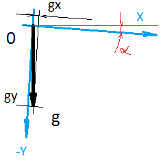
The task is as follows: we need to determine the zero displacement vector using the sensor readings, which will always record the displacement vector + constant external influence vector (gravitational acceleration, Earth rotation, Earth’s magnetic field), the magnitude and direction of which we do not know (in the case of the accelerometer we know the value, but again the scale of the sensor may not be equal to 1).
The way to solve. This article proposes to determine the displacement vector as follows. We take and twist the sensor in every way and register the sensor readings. After N measurements, the values taken from the sensor and located on the graph will represent a ball, the radius of which is the magnitude of the external influence, and the center is just the desired value of the zero offset.
To facilitate the measurement procedure itself, you can write a simple program. It should record the sensors when the device is stationary. We will only have to turn the device to the desired position. In order to determine a stationary state, an uncalibrated accelerometer is also suitable - just take the difference between the current value and the previous one. And if there is more noise, then we fix the movement. My threshold is in the region of 0.07G. If you hold with your hands, more than this value will turn out. I used masking tape to fix the position. If it still doesn’t work out, check to see if there is a fridge, fan, or something similar nearby.
To get the ball on the graph, you need to twist the device with the sensor according to a certain scheme. For these purposes, the globe is well suited, since it has a markup. You might think that you need to sculpt all over the globe. But this is not so.
It is necessary to sculpt the sensor not on the entire surface of the globe, but on one meridian. Suppose we take seven points on the meridian (the first and last at the north and south poles). At each point of the meridian we attach your device to the globe and still twist the device around its axis with a certain step, for example 30-35 degrees. It turns out if you rotate 12 times around its axis, then at 7 points in total 84 measurements are obtained.
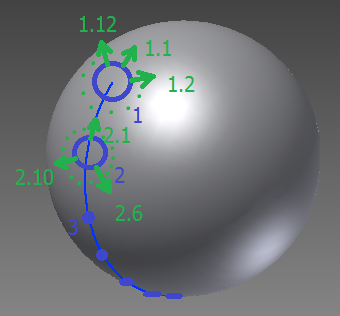
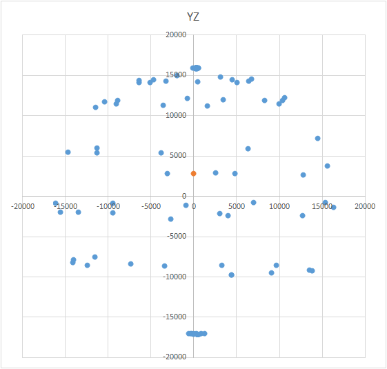
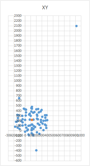
The beauty of the method is that everything can be done “on the knee”. Positioning accuracy does not play a special role, you just need to twist according to the scheme so that the vector of external influence on the graph draws a ball. The correct one looks something like this - see the figure (the center is marked with a mark).
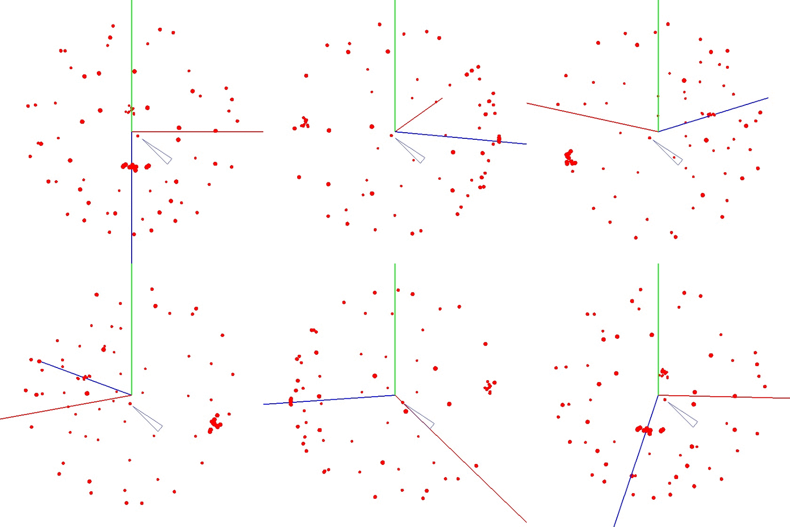
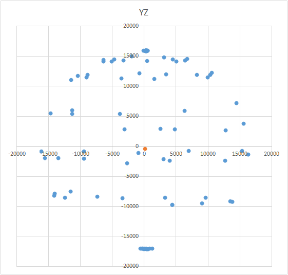
This is an interesting task and it has several solutions. It may seem that to search for the center, it is enough to take the arithmetic average of the coordinates of the obtained points. However, this is not so - the points can be located unevenly on the ball (see. Fig.).
The equation of the ball looks like this: (X - A) 2 + (Y - B) 2 + (Z - C) 2 = R 2 , where X, Y, Z are the coordinates of the point lying on the ball. A, B, C are the coordinates of the center on the x, y, and z axes, respectively. R is the radius of the ball. You can build a system of equations and try to solve this system more simply using some method. Or you can just bust to find the center (this is like a method of successive approximations). The meaning of the method is simple: the error value (X - A) 2 + (Y - B) 2+ (Z - C) 2 - R 2 should tend to zero. So, the sum of these values for all points of the sphere should also tend to zero. Knowing this, we can choose values A, B, and C for which the error value for all points will be minimal. The search area is limited by the size of the ball (conditional cube). That is, we must sequentially put the center of the ball at all points of the cube and calculate the error. Where there is minimal error - there is the center.
As R, we need to take the theoretical value of the vector of external influence - for the accelerometer, this is the acceleration of gravity, for the compass - this is the average magnitude of the Earth's magnetic field, for the gyroscope - the speed of rotation of the Earth. Of course, in the formula there should be values of one dimension (conventional units of the sensor or m / s 2, degrees / s, etc.). It is more convenient to convert to arbitrary units of the corresponding sensor.
By the way, if you know the radius of the ball exactly, then you can calculate the center only by its “wedge”. That is, at points that are located only on a piece of the surface of the ball. But this is not our case.
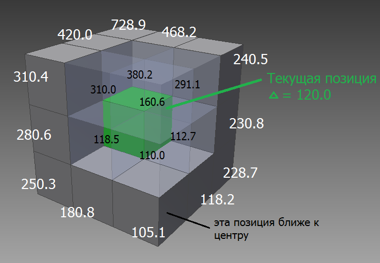
It is necessary to look for the center not in the whole cube (the dimensions of the ball), but in a line whose beginning is arbitrary, each next point is closer to the real center and the end is in the center. Suppose we start from the point (0; 0; 0) ... We always move with a constant step. Therefore, if we imagine a set of 3x3x3 cubes, where each face is equal to the step size and also imagine that the current position is the middle cube, then we have 9 + 8 + 9 options where to put the next point. We just have to be at each point, to calculate in which of the neighboring 26 points the error will be less. If it turns out that the error is less at the current point, and not at one of the neighboring ones, then it means that it is in the center and the search is over.
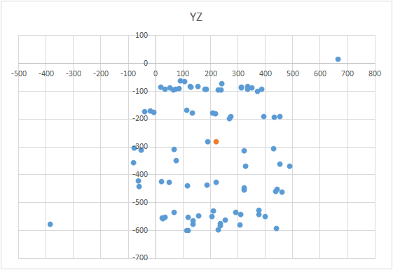
Need to search with variable pitch. First we look for the center in large steps. We found the center, we reduce the step and from it we begin to search further. And so on, until you get the result of the necessary accuracy.
During measurements, there may be situations when, for some reason, the measurement result may be much farther from the surface of the ball. Or it could be a lot of points. Or, in general, the result of measurements may not be a ball, but an “egg” or an “airship”. In this case, of course, you need to repeat all the measurements, identifying the possible causes of errors. For example, for a magnetometer, it can be a bolt or a nail in the table and you are taking measurements directly above it. And the lower you lower the sensor along the meridian, the stronger the metal will affect the result. Therefore, it is necessary to determine the threshold of the permissible error value. In order not to redo the measurements due to several obviously erroneous points, you can apply a filter. The principle of the filter is very simple - after calculating the center for the first time, sort the points by the error level in each of them. Some of the points with the largest error can simply be thrown away (for example, 10%). Then you need to repeat the search for the center.
The method has pretty good accuracy. The method allows you to do with simple improvised means (ball, bank, etc.). It works fast enough. Simple code. Many sensors have special registers where you can write the found value, and the sensor will subtract it on the fly. Such registers usually have the prefix “TRIM”, as in the MPU9260, or “OFFSET”, as in the LSM303. But the well-known LIS302DL does not have such registers.
Do not forget to put a plus sign if you liked it. Write in the comments your methods for calibrating sensors.

Publication structure
- Problem
- Statement of the problem and method of solution
- How to get the points?
- How to calculate the center of the ball?
- How to speed up the search for the center of the ball?
- How else to speed up the search for the center of the ball?
- About measurement errors
- Total
Problem
What is the problem - MEMS sensors after installation in the board undergo minor deformations that affect:
- zero position;
- scaling of measured values;
- perpendicularity of axes to each other.
And if scaling and perpendicularity are violated not so noticeably, then the zero position gets tangled up significantly. For example, if you translate the typical value of the zero offset for the accelerometer of the MPU9250 sensor into m / s 2 , then this is obtained in the region of 0.2 m / s 2 . That is, the sensor is stationary, but it shows acceleration, and after 5 seconds we get a speed of 1 m / s. On the one hand, all sensor data is always passed through a filter (for example, such ). But on the other hand, why should the filter constantly compensate for this bias? After all, the sensor will show movement where it is not. This reduces the accuracy of the result. All in all, you need to find the offset value once and then subtract this value from its readings during sensor operation.
The simplest solution to finding the value of the zero offset, which immediately comes to mind, is to create the conditions under which the sensor must accurately show zero. The value recorded on the sensor is the value of the zero offset! So? But no - gravity is constantly acting on the accelerometer. To avoid it, weightlessness will be needed (tossing will not work). The Earth’s magnetic field acts on the compass, and its rotation on the gyroscope. So, if you do not have a personal starship, then you have to come up with something.
The second solution that immediately comes to mind is to put the sensor (or rather its axis) in a position in which we will know exactly what the sensor should show. The difference between what the sensor shows and what it should show - and there will be a zero offset! So? For example, we know that if the accelerometer is placed in a level with the horizon, then in theory, the gravitational acceleration vector will be directed exactly along the Z axis of the sensor. The magnitude of the acceleration vector we know.
However, there is a problem. It consists in the fact that we cannot precisely set the axis of the sensor to a level with the horizon. The fact is that the surface on which we will rely is not parallel to the printed circuit board. That, in turn, is not parallel to the site on which the sensor is located. The sensor itself does not stand exactly on its site and the axes inside the sensor are not parallel to the sensor body. The error in setting the axis relative to the horizon by 1 degree gives a projection comparable in size to the value of the zero offset itself, which we want to find. In the case of a magnetometer, we also do not know where the magnetic field vector is directed. In theory, to the north. But in practice, the Earth’s magnetic field itself is heterogeneous in intensity and direction. Plus, the nearest metal objects make their adjustments.

Statement of the problem and method of solution
The task is as follows: we need to determine the zero displacement vector using the sensor readings, which will always record the displacement vector + constant external influence vector (gravitational acceleration, Earth rotation, Earth’s magnetic field), the magnitude and direction of which we do not know (in the case of the accelerometer we know the value, but again the scale of the sensor may not be equal to 1).
The way to solve. This article proposes to determine the displacement vector as follows. We take and twist the sensor in every way and register the sensor readings. After N measurements, the values taken from the sensor and located on the graph will represent a ball, the radius of which is the magnitude of the external influence, and the center is just the desired value of the zero offset.
How to get the points?
To facilitate the measurement procedure itself, you can write a simple program. It should record the sensors when the device is stationary. We will only have to turn the device to the desired position. In order to determine a stationary state, an uncalibrated accelerometer is also suitable - just take the difference between the current value and the previous one. And if there is more noise, then we fix the movement. My threshold is in the region of 0.07G. If you hold with your hands, more than this value will turn out. I used masking tape to fix the position. If it still doesn’t work out, check to see if there is a fridge, fan, or something similar nearby.
How can it be in code
// здесь у вас глобальные по модулю переменные
static TSumSensorsData 	g_sens_data[2];
static int32_t   	g_sens_data_sum_cnt[2];
static uint8_t		g_sens_data_num;
// здесь какое-то прерывание, при получении данных с датчиков
IS_INTERRUPT void on_dma_raw_ready_calibrate_step1()
{
	SensorRawBuffer *raw = sensor_get_raw_buffer();
	g_sens_data[g_sens_data_num].acc_x += swap_i16(raw->accell_x_unswap);
	g_sens_data[g_sens_data_num].acc_y += swap_i16(raw->accell_y_unswap);
	g_sens_data[g_sens_data_num].acc_z += swap_i16(raw->accell_z_unswap);
	g_sens_data[g_sens_data_num].gyro_x += swap_i16(raw->gyro_x_unswap);
	g_sens_data[g_sens_data_num].gyro_y += swap_i16(raw->gyro_y_unswap);
	g_sens_data[g_sens_data_num].gyro_z += swap_i16(raw->gyro_z_unswap);
	g_sens_data[g_sens_data_num].mag_x += raw->mag_x_raw * g_mag_calibrate.kx;
	g_sens_data[g_sens_data_num].mag_y += raw->mag_y_raw * g_mag_calibrate.ky;
	g_sens_data[g_sens_data_num].mag_z += raw->mag_z_raw * g_mag_calibrate.kz;
	g_sens_data_sum_cnt[g_sens_data_num]++;
}
//это вызывается из main
void sensors_calibrate_program(FlashROM *flash_ptr)
{
	double calibrate_result_error[3];
	TVector16 calibrate_result[3];
	int32_t radius[ACCEL_NO_MOTION_DETECT_COUNT];
	uint8_t raw_is_deleted[ACCEL_NO_MOTION_DETECT_COUNT];
	TVector16 raw[3][ACCEL_NO_MOTION_DETECT_COUNT];
        . . .
	// определяю неподвижность
	g_sens_data_sum_cnt[0] = 0;
	g_sens_data_num = 0;
	int16_t prev_avg_x = 0;
	int16_t prev_avg_y = 0;
	int16_t prev_avg_z = 0;
	int8_t low_motion_cnt = 0;
	while(low_motion_cnt < ACCEL_NO_MOTION_DETECT_COUNT)
	{
		if (g_sens_data_sum_cnt[g_sens_data_num] >= ACCEL_NO_MOTION_DETECT_SAMPLES)
		{
			uint8_t new_data_num = (g_sens_data_num + 1) & 1;
			g_sens_data[new_data_num].acc_x = 0;
			g_sens_data[new_data_num].acc_y = 0;
			g_sens_data[new_data_num].acc_z = 0;
			g_sens_data[new_data_num].gyro_x = 0;
			g_sens_data[new_data_num].gyro_y = 0;
			g_sens_data[new_data_num].gyro_z = 0;
			g_sens_data[new_data_num].mag_x = 0;
			g_sens_data[new_data_num].mag_y = 0;
			g_sens_data[new_data_num].mag_z = 0;
			g_sens_data_sum_cnt[new_data_num] = 0;
			uint8_t old_data_num = g_sens_data_num;
			g_sens_data_num = new_data_num; // вот эта операция не может быть выполнена во время работы прерывания
			// (так по-простому можно разделить два потока, не имея операционки)
			// здесь всё очень просто - нахожу среднюю
			int16_t avg_x = g_sens_data[old_data_num].acc_x / g_sens_data_sum_cnt[old_data_num];
			int16_t avg_y = g_sens_data[old_data_num].acc_y / g_sens_data_sum_cnt[old_data_num];
			int16_t avg_z = g_sens_data[old_data_num].acc_z / g_sens_data_sum_cnt[old_data_num];
			// собственно получаю разницу с предыдущим значением
			int16_t dx = avg_x - prev_avg_x;
			int16_t dy = avg_y - prev_avg_y;
			int16_t dz = avg_z - prev_avg_z;
			prev_avg_x = avg_x;
			prev_avg_y = avg_y;
			prev_avg_z = avg_z;
			// если акселерометр регистрировал низкую активность
			if ((abs_i16(dx) <= ACCEL_NO_MOTION_DETECT_AVG_VALUE)&&(abs_i16(dy) <= ACCEL_NO_MOTION_DETECT_AVG_VALUE)&&(abs_i16(dz) <= ACCEL_NO_MOTION_DETECT_AVG_VALUE))
			{
				// тогда мы регистрируем точку
				raw[RAW_ACC][low_motion_cnt].x = avg_x;
				raw[RAW_ACC][low_motion_cnt].y = avg_y;
				raw[RAW_ACC][low_motion_cnt].z = avg_z;
				raw[RAW_GYRO][low_motion_cnt].x = g_sens_data[old_data_num].gyro_x / g_sens_data_sum_cnt[old_data_num];
				raw[RAW_GYRO][low_motion_cnt].y = g_sens_data[old_data_num].gyro_y / g_sens_data_sum_cnt[old_data_num];
				raw[RAW_GYRO][low_motion_cnt].z = g_sens_data[old_data_num].gyro_z / g_sens_data_sum_cnt[old_data_num];
				raw[RAW_MAG][low_motion_cnt].x = g_sens_data[old_data_num].mag_x / g_sens_data_sum_cnt[old_data_num];
				raw[RAW_MAG][low_motion_cnt].y = g_sens_data[old_data_num].mag_y / g_sens_data_sum_cnt[old_data_num];
				raw[RAW_MAG][low_motion_cnt].z = g_sens_data[old_data_num].mag_z / g_sens_data_sum_cnt[old_data_num];
				low_motion_cnt++;
				// даём звуковой сигнал
				beep();
				// и даём фору себе 2 секунды отклеить скотч, пока датчик в руках - программа регистрирует движение
				// прилепили - получили точку
				// поэтому всё получится быстро и весело
				delay_ms(2000);
			}
		}
	}
. . .
}
To get the ball on the graph, you need to twist the device with the sensor according to a certain scheme. For these purposes, the globe is well suited, since it has a markup. You might think that you need to sculpt all over the globe. But this is not so.
Wrong result example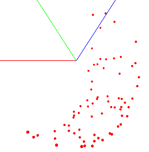

It is necessary to sculpt the sensor not on the entire surface of the globe, but on one meridian. Suppose we take seven points on the meridian (the first and last at the north and south poles). At each point of the meridian we attach your device to the globe and still twist the device around its axis with a certain step, for example 30-35 degrees. It turns out if you rotate 12 times around its axis, then at 7 points in total 84 measurements are obtained.

The beauty of the method is that everything can be done “on the knee”. Positioning accuracy does not play a special role, you just need to twist according to the scheme so that the vector of external influence on the graph draws a ball. The correct one looks something like this - see the figure (the center is marked with a mark).

How to calculate the center of the ball?
This is an interesting task and it has several solutions. It may seem that to search for the center, it is enough to take the arithmetic average of the coordinates of the obtained points. However, this is not so - the points can be located unevenly on the ball (see. Fig.).

The equation of the ball looks like this: (X - A) 2 + (Y - B) 2 + (Z - C) 2 = R 2 , where X, Y, Z are the coordinates of the point lying on the ball. A, B, C are the coordinates of the center on the x, y, and z axes, respectively. R is the radius of the ball. You can build a system of equations and try to solve this system more simply using some method. Or you can just bust to find the center (this is like a method of successive approximations). The meaning of the method is simple: the error value (X - A) 2 + (Y - B) 2+ (Z - C) 2 - R 2 should tend to zero. So, the sum of these values for all points of the sphere should also tend to zero. Knowing this, we can choose values A, B, and C for which the error value for all points will be minimal. The search area is limited by the size of the ball (conditional cube). That is, we must sequentially put the center of the ball at all points of the cube and calculate the error. Where there is minimal error - there is the center.

As R, we need to take the theoretical value of the vector of external influence - for the accelerometer, this is the acceleration of gravity, for the compass - this is the average magnitude of the Earth's magnetic field, for the gyroscope - the speed of rotation of the Earth. Of course, in the formula there should be values of one dimension (conventional units of the sensor or m / s 2, degrees / s, etc.). It is more convenient to convert to arbitrary units of the corresponding sensor.
How to calculate a certain value in the standard units of the sensor?
Conventional units of the sensor = Value * Resolution of the sensor / (Maximum measurement limit - Minimum measurement limit)
For example: How many conventional units should a 16-bit acceleration sensor with a measurement limit of ± 2g show when the sensor is exposed to only gravity acceleration ?:
9.8 m / s 2 * 65536 / (2g + 2g) = 9.8 m / s 2 * 65536 / (2 * 9.8 m / s 2 + 2 * 9.8 m / s 2 ) = 16384 y. e. sensor.
For example: How many conventional units should a 16-bit acceleration sensor with a measurement limit of ± 2g show when the sensor is exposed to only gravity acceleration ?:
9.8 m / s 2 * 65536 / (2g + 2g) = 9.8 m / s 2 * 65536 / (2 * 9.8 m / s 2 + 2 * 9.8 m / s 2 ) = 16384 y. e. sensor.
By the way, if you know the radius of the ball exactly, then you can calculate the center only by its “wedge”. That is, at points that are located only on a piece of the surface of the ball. But this is not our case.
How to speed up the search for the center of the ball?
It is necessary to look for the center not in the whole cube (the dimensions of the ball), but in a line whose beginning is arbitrary, each next point is closer to the real center and the end is in the center. Suppose we start from the point (0; 0; 0) ... We always move with a constant step. Therefore, if we imagine a set of 3x3x3 cubes, where each face is equal to the step size and also imagine that the current position is the middle cube, then we have 9 + 8 + 9 options where to put the next point. We just have to be at each point, to calculate in which of the neighboring 26 points the error will be less. If it turns out that the error is less at the current point, and not at one of the neighboring ones, then it means that it is in the center and the search is over.

How can it be in code
Public Function get_err(A As Double, B As Double, C As Double, R As Double) As Double
Dim x, y, z As Double
Dim sigma As Double
Dim row_n As Long
get_err = 0
For row_n = 1 To 15
    x = Application.ActiveWorkbook.ActiveSheet.Cells(row_n, 1).Value
    y = Application.ActiveWorkbook.ActiveSheet.Cells(row_n, 2).Value
    z = Application.ActiveWorkbook.ActiveSheet.Cells(row_n, 3).Value
    get_err = get_err + abs( (A - x) ^ 2 + (B - y) ^ 2 + (C - z) ^ 2 - R ^ 2 )
Next
End Function
. . .
A = 0
B = 0
C = 0
Do While True
   min_sigma = 0
    For ai = -1 To 1
        For bi = -1 To 1
            For ci = -1 To 1
                sigma = get_err(A + ai, B + bi, C + ci, 16384)
                If sigma < min_sigma Or min_sigma = 0 Then
                    ai_min = ai
                    bi_min = bi
                    ci_min = ci
                    min_sigma = sigma
                End If
            Next
        Next
    Next
    If ai_min = 0 And bi_min = 0 And ci_min = 0 Then
        Exit Do
    End If
    A = A + ai_min
    B = B + bi_min
    C = C + ci_min
Loop
. . .
How else to speed up the search for the center of the ball?
Need to search with variable pitch. First we look for the center in large steps. We found the center, we reduce the step and from it we begin to search further. And so on, until you get the result of the necessary accuracy.
How can it be in code
Public Function get_err(A As Double, B As Double, C As Double, R As Double) As Double
Dim x, y, z As Double
Dim sigma As Double
Dim row_n As Long
get_err = 0
For row_n = 1 To 15
    x = Application.ActiveWorkbook.ActiveSheet.Cells(row_n, 1).Value
    y = Application.ActiveWorkbook.ActiveSheet.Cells(row_n, 2).Value
    z = Application.ActiveWorkbook.ActiveSheet.Cells(row_n, 3).Value
    get_err = get_err + abs( (A - x) ^ 2 + (B - y) ^ 2 + (C - z) ^ 2 - R ^ 2 )
Next
End Function
. . .
A = 0
B = 0
C = 0
step = 1000
Do While True
   min_sigma = 0
    For ai = -1 To 1
        For bi = -1 To 1
            For ci = -1 To 1
                sigma = get_err(A + ai * step, B + bi * step, C + ci * step, 16384)
                If sigma < min_sigma Or min_sigma = 0 Then
                    ai_min = ai
                    bi_min = bi
                    ci_min = ci
                    min_sigma = sigma
                End If
            Next
        Next
    Next
    If ai_min = 0 And bi_min = 0 And ci_min = 0 Then
        step = step / 10
        If step < 0.01 Then
            Exit Do
        End If
    Else
    A = A + ai_min * step
    B = B + bi_min * step
    C = C + ci_min * step
    End If
Loop
. . .
About measurement errors
During measurements, there may be situations when, for some reason, the measurement result may be much farther from the surface of the ball. Or it could be a lot of points. Or, in general, the result of measurements may not be a ball, but an “egg” or an “airship”. In this case, of course, you need to repeat all the measurements, identifying the possible causes of errors. For example, for a magnetometer, it can be a bolt or a nail in the table and you are taking measurements directly above it. And the lower you lower the sensor along the meridian, the stronger the metal will affect the result. Therefore, it is necessary to determine the threshold of the permissible error value. In order not to redo the measurements due to several obviously erroneous points, you can apply a filter. The principle of the filter is very simple - after calculating the center for the first time, sort the points by the error level in each of them. Some of the points with the largest error can simply be thrown away (for example, 10%). Then you need to repeat the search for the center.


Total
The method has pretty good accuracy. The method allows you to do with simple improvised means (ball, bank, etc.). It works fast enough. Simple code. Many sensors have special registers where you can write the found value, and the sensor will subtract it on the fly. Such registers usually have the prefix “TRIM”, as in the MPU9260, or “OFFSET”, as in the LSM303. But the well-known LIS302DL does not have such registers.
Do not forget to put a plus sign if you liked it. Write in the comments your methods for calibrating sensors.
