Generative adversarial networks
In the last article, we looked at the simplest linear generative PPCA model. The second generative model we will look at is the Generative Adversarial Networks, abbreviated GAN. In this article, we will consider the most basic version of this model, leaving advanced versions and comparisons with other approaches in generative modeling to the next chapters.
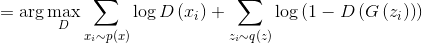
Generative modeling involves the approximation of uncalculated posterior distributions. Because of this, most effective methods developed for training discriminatory models do not work with generative models. Existing methods for solving this problem are computationally difficult and are mainly based on the use of Markov Chain Monte Carlo , which is poorly scalable. Therefore, to train generative models, we needed a method based on scalable techniques such as Stochastic Gradient Descent (SGD) and backpropagation . One such method is Generative Adversarial Networks (GAN). GANs were first proposed in thisarticle in 2014. High-level this model can be described as two submodels that compete with each other, and one of these models (generator), is trying to learn in a sense to deceive the second (discriminator). To do this, the generator generates random objects, and the discriminator tries to distinguish these generated objects from real objects from the training set. In the learning process, the generator generates more and more similar objects to the sample, and it becomes increasingly difficult for the discriminator to distinguish them from the real ones. Thus, the generator turns into a generative model that generates objects from some complex distribution, for example, from the distribution of photographs of human faces.
First, we introduce the necessary terminology. Through we will denote some space of objects. For example,
  pixel pictures . A
  vector random variable
  with a probability distribution having a density
  such that a subset of the space on which it takes nonzero values is, for example, photographs of human faces, given a probability space . We are given a random iid sample of face photos for magnitude
  . Additionally, we define an auxiliary space
  and a random variable
  with a probability distribution having a density
  .
.  - discriminator function. This function takes an object as input.
 (in our example, a picture of the appropriate size) and returns the probability that the input picture is a photograph of a human face.
  - generator function. It takes on value
  and gives out an object of space , that is, in our case, a picture.
Suppose we already have a perfect discriminator . For any example,
  it gives the true probability that this example belongs to the given subset from which the sample is derived
  . Reformulating the problem of deceiving the discriminator in a probabilistic language, we find that it is necessary to maximize the probability generated by the ideal discriminator on the generated examples. Thus, the optimal generator is found as
  . Because
 - a monotonously increasing function and does not change the position of the extrema of the argument, rewrite this formula in the form
  that will be convenient in the future.
In reality, there is usually no ideal discriminator and must be found. Since the task of the discriminator is to provide a signal for training the generator, instead of the ideal discriminator, it is enough to take a discriminator that ideally separates the real examples from those generated by the current generator, i.e. ideal only on the subsetfrom which examples are generated by the current generator. This problem can be reformulated as the search for such a function, which maximizes the likelihood of correctly classifying the examples as real or generated. This is called the binary classification problem, and in this case we have an infinite training set: a finite number of real examples and a potentially infinite number of generated examples. Each example has a label: whether it is real or generated. The first article described a solution to the classification problem using the maximum likelihood method. Let's write it for our case.
So, our sample . We define the distribution density
  , then
  this is a reformulation of the discriminator that gives the probability of a class
  (a real example) in the form of a distribution on classes
  . Because
 , this definition sets the correct probability density. Then the optimal discriminator can be found as:

Group the factors for and
and  :
:
And when the sample size tends to infinity, we get:

Total, we get the following iterative process:
In the original article, this algorithm is summarized into one formula that defines, in a sense, the minimax game between the discriminator and the generator:

Both functions can be represented in the form of neural networks:
  after which the task of finding optimal functions is reduced to the problem of optimization by parameters and it can be solved using traditional methods: backpropagation and SGD. Additionally, since the neural network is a universal approximator of functions, it
  can approximate an arbitrary probability distribution, which removes the question of the choice of distribution . It can be any continuous distribution within some reasonable framework. For example,
  or
or  . The correctness of this algorithm and its convergence
  to under fairly general assumptions is proved in the original article.
We figured out the math, let's now see how it works. Suppose , i.e. we solve a one-dimensional problem.
  . Let's use a linear generator
 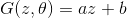 where
where  . The discriminator will be a fully connected three-layer neural network with a binary classifier at the end. The solution to this problem is
  , that is
  . Now let's try to program a numerical solution to this problem using Tensorflow. The full code can be found here , but only key points are covered in the article.
The first thing to ask is input sample: . Since the training is in minibatches, we will generate a vector of numbers at a time. Additionally, the sample is parameterized by the mean and standard deviation.
Now let's set random inputs for the generator :
:
Define a generator. We take the absolute value of the second parameter to give it the meaning of the standard deviation:
Let's create a vector of real examples:
And the vector of generated examples:
Now let's run all the examples through the discriminator. It is important to remember that we do not want two different discriminators, but one, because Tensorflow needs to be asked to use the same parameters for both inputs:
The loss function in real examples is the cross-entropy between the unit (the expected response of the discriminator in real examples) and discriminator estimates:
The loss function on fake examples is the cross-entropy between zero (expected discriminator response on fake examples) and discriminator estimates:
The discriminator loss function is the sum of losses on real examples and fake examples:
The generator loss function is the cross-entropy between the unit (the desired discriminator error response on fake examples) and the estimates of these fake examples by the discriminator:
An optional L2 regularization is added to the discriminator loss function.
Model training is reduced to sequential training of the discriminator and generator in a cycle until convergence:
Below are the graphs for the four discriminator models:

Fig. 1. The probability that the discriminator classifies the real example as real.

Fig. 2. The probability of classification by the discriminator of the generated example as real.
All four models quickly converge to what the discriminator produces at all inputs. Due to the simplicity of the problem that the generator solves, there is almost no difference between the models. The graphs show that the mean and standard deviation quickly converge to the values from the data distribution:

Fig. 3. The average of the generated distributions.
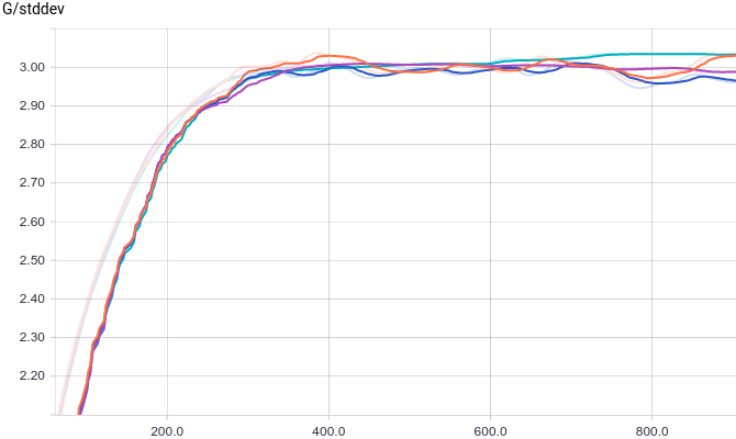
Fig. 4. The standard deviation of the generated distributions.
Below are the distributions of the actual and generated examples in the learning process. It can be seen that the generated examples by the end of the training are practically indistinguishable from the real ones (they are distinguished on the graphs because Tensorboard chose different scales, but if you look at the values, they are the same).

Fig. 5. Distribution of real data. Does not change over time. The training step is delayed on the vertical axis.


Fig. 6. Distribution of real data. Does not change over time. The training step is delayed on the vertical axis.
Let's look at the model training process:
Fig. 7. Visualization of the learning process of the model. Fixed Gaussian - distribution density of real data, moving Gaussian - distribution density of generated examples, the blue curve is the result of the discriminator, i.e. the likelihood of an example being real.
It can be seen that the discriminator at the beginning of training separates the data very well, but the distribution of the generated examples very quickly literally “creeps” to the distribution of the real examples. In the end, the generator approximates the data so well that the discriminator becomes a constantand the task converges.
Let’s try to replacewith  , thereby simulating the multimodal distribution of the source data. For this model, only the code for generating real examples needs to be changed. Instead of returning a normally distributed random variable, we return a mixture of several:
Below are the graphs for the same models as in the previous experiment, but for data with two modes:

Fig. 8. The probability of classification by a discriminator of a real example as a real one.
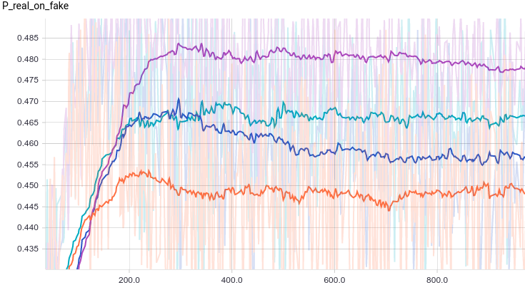
Fig. 9. The probability of classification by the discriminator of the generated example as real.
It is interesting to note that regularized models show themselves significantly better than irregularized ones. However, regardless of the model, it is clear that now the generator fails to fool the discriminator so well. Let’s understand why it happened.

Fig. 10. The average of the generated distributions.

Fig. 11. The standard deviation of the generated distributions.
As in the first experiment, the generator approximates the data with a normal distribution. The reason for the decline in quality is that now the data cannot be accurately approximated by a normal distribution, because they are sampled from a mixture of two normal ones. The modes of the mixture are symmetrical with respect to zero, and it can be seen that all four models approximate the data by a normal distribution with a center near zero and a sufficiently large dispersion. Let's look at the distribution of real and fake examples to understand what happens:

Figure 12. Distribution of real data. Does not change over time. The training step is delayed on the vertical axis.
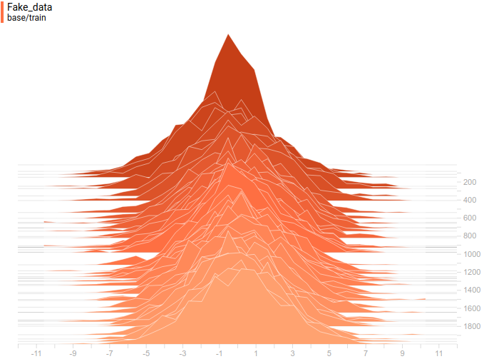


Figure 13. Distributions of generated data from four models. The training step is delayed on the vertical axis.
This is how the model learning process goes:
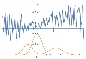
Fig. 14. Visualization of the learning process of the model. A fixed Gaussian mixture is the distribution density of real data, a moving Gaussian is the distribution density of the generated examples, the blue curve is the result of the discriminator, i.e. the likelihood of an example being real.
This animation shows in detail the case studied above. The generator, not possessing sufficient expressiveness and being able to approximate data only by a Gaussian, spreads out into a wide Gaussian, trying to cover both modes of data distribution. As a result, the generator reliably deceives the discriminator only in places where the areas under the generator curves and the source data are close, that is, at the intersection of these curves.
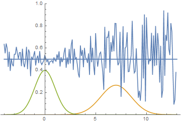
However, this is not the only possible case. Let's move the right mode a little to the right, so that the initial approximation of the generator does not capture it.
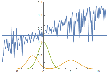
Fig. 15. Visualization of the model learning process. A fixed Gaussian mixture is the distribution density of real data, a moving Gaussian is the distribution density of the generated examples, the blue curve is the result of the discriminator, i.e. the likelihood of an example being real.
It is seen that in this case it is most profitable for the generator to try to approximate the left distribution mode. After this happens, the generator tries to attempt to capture the left mode. It looks like oscillations of the standard deviation of the generator in the second half of the animation. But all these attempts fail, because the discriminator “locks” the generator and, in order to capture the left mode, it needs to overcome the barrier from the high loss function, which it cannot do because of the insufficiently high learning speed. This effect is called mode collapse.
In the two examples described above, we saw two types of problems that arise if the generator is not powerful enough to express the initial distribution of data: mode averaging, when the generator approximates the entire distribution, but everywhere is bad enough; and mode collapse, when a generator learns a subset of modes, and those that it has not learned do not affect it in any way.
In addition to the fact that both of these problems lead to the discriminator k being inconsistent, they also lead to a decrease in the quality of the generative model. The first problem leads to the fact that the generator gives examples “between” modes, which should not be, the second problem leads to the fact that the generator gives examples only from some modes, thereby reducing the richness of the initial data distribution.
The reason that the previous section could not completely deceive the discriminator was the triviality of the generator, which simply did a linear transformation. Now let's try to use a fully-connected three-layer neural network as a generator:
Let's look at the training schedules.

Fig. 16. The probability of classification by the discriminator of a real example as a real one.

Fig. 17. The probability of classification by the discriminator of the generated example as real.
It can be seen that due to the large number of parameters, training has become much more noisy. The discriminators of all models converge to a result of about, but they behave unstably around this point. Let's look at the shape of the generator.
Figure 18. Distribution of real data. Does not change over time. The training step is delayed on the vertical axis.


Figure 19. Distributions of generated data from four models. The training step is delayed on the vertical axis.
It can be seen that the distribution of the generator, although it does not coincide with the distribution of data, is quite similar to it. The most regularized model again proved to be the best. It can be seen that she learned two modes that roughly coincide with the data distribution modes. Peak sizes are also not very accurate, but approximate the distribution of data. Thus, a neural network generator is able to learn the multimodal data distribution.
This is how the model learning process goes:
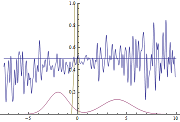
Fig. 20. Visualization of the learning process of a model with close modes. A fixed Gaussian mixture is the distribution density of real data, a moving Gaussian is the distribution density of the generated examples, the blue curve is the result of the discriminator, i.e. the likelihood of an example being real.
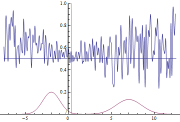
Fig. 21. Visualization of the learning process of the model with distant modes. A fixed Gaussian mixture is the distribution density of real data, a moving Gaussian is the distribution density of the generated examples, the blue curve is the result of the discriminator, i.e. the likelihood of an example being real.
These two animations show training on data distributions from the previous section. It can be seen from these animations that when using a sufficiently large generator with many parameters, it, although quite roughly, is able to approximate the multimodal distribution, thereby indirectly confirming that the problems from the previous section arise due to an insufficiently complex generator. The discriminators on these animations are much noisier than in the section on finding the parameters of the normal distribution, but, nevertheless, by the end of the training they begin to resemble a noisy horizontal line .
.
GAN is a model for approximating an arbitrary distribution only by sampling from this distribution. In this article, we looked in detail how the model works on a trivial example of searching for parameters of a normal distribution and on a more complex example of approximating a bimodal distribution by a neural network. Both problems were solved with good accuracy, for which it was only necessary to use a rather complex model of the generator. In the next article, we will move from these model examples to real examples of generating samples from complex distributions using the example of image distribution.
Thanks to Olga Talanova and Ruslan Login for reviewing the text. Thanks to Ruslan Login for help in preparing images and animations. Thanks to Andrei Tarashkevich for helping with the layout of this article.
History
Generative modeling involves the approximation of uncalculated posterior distributions. Because of this, most effective methods developed for training discriminatory models do not work with generative models. Existing methods for solving this problem are computationally difficult and are mainly based on the use of Markov Chain Monte Carlo , which is poorly scalable. Therefore, to train generative models, we needed a method based on scalable techniques such as Stochastic Gradient Descent (SGD) and backpropagation . One such method is Generative Adversarial Networks (GAN). GANs were first proposed in thisarticle in 2014. High-level this model can be described as two submodels that compete with each other, and one of these models (generator), is trying to learn in a sense to deceive the second (discriminator). To do this, the generator generates random objects, and the discriminator tries to distinguish these generated objects from real objects from the training set. In the learning process, the generator generates more and more similar objects to the sample, and it becomes increasingly difficult for the discriminator to distinguish them from the real ones. Thus, the generator turns into a generative model that generates objects from some complex distribution, for example, from the distribution of photographs of human faces.
Model
First, we introduce the necessary terminology. Through
we will denote some space of objects. For example, pixel pictures . A vector random variable with a probability distribution having a density such that a subset of the space on which it takes nonzero values is, for example, photographs of human faces, given a probability space . We are given a random iid sample of face photos for magnitude . Additionally, we define an auxiliary space and a random variable with a probability distribution having a density . - discriminator function. This function takes an object as input.(in our example, a picture of the appropriate size) and returns the probability that the input picture is a photograph of a human face. - generator function. It takes on value and gives out an object of space , that is, in our case, a picture. Suppose we already have a perfect discriminator
. For any example, it gives the true probability that this example belongs to the given subset from which the sample is derived . Reformulating the problem of deceiving the discriminator in a probabilistic language, we find that it is necessary to maximize the probability generated by the ideal discriminator on the generated examples. Thus, the optimal generator is found as . Because- a monotonously increasing function and does not change the position of the extrema of the argument, rewrite this formula in the form that will be convenient in the future. In reality, there is usually no ideal discriminator and must be found. Since the task of the discriminator is to provide a signal for training the generator, instead of the ideal discriminator, it is enough to take a discriminator that ideally separates the real examples from those generated by the current generator, i.e. ideal only on the subset
from which examples are generated by the current generator. This problem can be reformulated as the search for such a function, which maximizes the likelihood of correctly classifying the examples as real or generated. This is called the binary classification problem, and in this case we have an infinite training set: a finite number of real examples and a potentially infinite number of generated examples. Each example has a label: whether it is real or generated. The first article described a solution to the classification problem using the maximum likelihood method. Let's write it for our case. So, our sample
. We define the distribution density , then this is a reformulation of the discriminator that gives the probability of a class (a real example) in the form of a distribution on classes . Because, this definition sets the correct probability density. Then the optimal discriminator can be found as:Group the factors for
and :And when the sample size tends to infinity, we get:
Total, we get the following iterative process:
- Set an arbitrary initial one
 .
. - The
 iteration begins
  .
. - We are looking for the best for the current generator discriminator:
 .
. - Improving the generator using the best discriminator:
 . It is important to be in the vicinity of the current generator. If you move away from the current generator, the discriminator will cease to be optimal and the algorithm will cease to be true.
 - The task of training the generator is considered solved when
 for anyone . If the process does not converge, then go to the next iteration in paragraph (2).
In the original article, this algorithm is summarized into one formula that defines, in a sense, the minimax game between the discriminator and the generator:
Both functions
can be represented in the form of neural networks: after which the task of finding optimal functions is reduced to the problem of optimization by parameters and it can be solved using traditional methods: backpropagation and SGD. Additionally, since the neural network is a universal approximator of functions, it can approximate an arbitrary probability distribution, which removes the question of the choice of distribution . It can be any continuous distribution within some reasonable framework. For example, or . The correctness of this algorithm and its convergence to under fairly general assumptions is proved in the original article.Finding normal distribution parameters
We figured out the math, let's now see how it works. Suppose
, i.e. we solve a one-dimensional problem. . Let's use a linear generator where . The discriminator will be a fully connected three-layer neural network with a binary classifier at the end. The solution to this problem is , that is . Now let's try to program a numerical solution to this problem using Tensorflow. The full code can be found here , but only key points are covered in the article. The first thing to ask is input sample:
. Since the training is in minibatches, we will generate a vector of numbers at a time. Additionally, the sample is parameterized by the mean and standard deviation.def data_batch(hparams):
"""
Input data are just samples from N(mean, stddev).
"""
return tf.random_normal(
[hparams.batch_size, 1], hparams.input_mean, hparams.input_stddev)
Now let's set random inputs for the generator
:def generator_input(hparams):
"""
Generator input data are just samples from N(0, 1).
"""
return tf.random_normal([hparams.batch_size, 1], 0., 1.)
Define a generator. We take the absolute value of the second parameter to give it the meaning of the standard deviation:
def generator(input, hparams):
  mean = tf.Variable(tf.constant(0.))
  stddev = tf.sqrt(tf.Variable(tf.constant(1.)) ** 2)
  return input * stddev + mean
Let's create a vector of real examples:
generator_input = generator_input(hparams)
generated = generator(generator_input)
And the vector of generated examples:
generator_input = generator_input(hparams)
generated = generator(generator_input)
Now let's run all the examples through the discriminator. It is important to remember that we do not want two different discriminators, but one, because Tensorflow needs to be asked to use the same parameters for both inputs:
with tf.variable_scope("discriminator"):
  real_ratings = discriminator(real_input, hparams)
with tf.variable_scope("discriminator", reuse=True):
  generated_ratings = discriminator(generated, hparams)
The loss function in real examples is the cross-entropy between the unit (the expected response of the discriminator in real examples) and discriminator estimates:
loss_real = tf.reduce_mean(
  tf.nn.sigmoid_cross_entropy_with_logits(
    labels=tf.ones_like(real_ratings),
    logits=real_ratings))
The loss function on fake examples is the cross-entropy between zero (expected discriminator response on fake examples) and discriminator estimates:
loss_generated = tf.reduce_mean(
  tf.nn.sigmoid_cross_entropy_with_logits(
    labels=tf.zeros_like(generated_ratings),
    logits=generated_ratings))
The discriminator loss function is the sum of losses on real examples and fake examples:
discriminator_loss = loss_generated + loss_real
The generator loss function is the cross-entropy between the unit (the desired discriminator error response on fake examples) and the estimates of these fake examples by the discriminator:
generator_loss = tf.reduce_mean(
  tf.nn.sigmoid_cross_entropy_with_logits(
    labels=tf.ones_like(generated_ratings),
    logits=generated_ratings))
An optional L2 regularization is added to the discriminator loss function.
Model training is reduced to sequential training of the discriminator and generator in a cycle until convergence:
for step in range(args.max_steps):
  session.run(model.discriminator_train)
  session.run(model.generator_train)
Below are the graphs for the four discriminator models:
- three-layer neural network.
- three-layer neural network with L2-regularization ..
- three-layer neural network with dropout-regularization.
- a three-layer neural network with L2 and dropout regularization.
Fig. 1. The probability that the discriminator classifies the real example as real.
Fig. 2. The probability of classification by the discriminator of the generated example as real.
All four models quickly converge to what the discriminator produces
at all inputs. Due to the simplicity of the problem that the generator solves, there is almost no difference between the models. The graphs show that the mean and standard deviation quickly converge to the values from the data distribution:Fig. 3. The average of the generated distributions.
Fig. 4. The standard deviation of the generated distributions.
Below are the distributions of the actual and generated examples in the learning process. It can be seen that the generated examples by the end of the training are practically indistinguishable from the real ones (they are distinguished on the graphs because Tensorboard chose different scales, but if you look at the values, they are the same).
Fig. 5. Distribution of real data. Does not change over time. The training step is delayed on the vertical axis.
Fig. 6. Distribution of real data. Does not change over time. The training step is delayed on the vertical axis.
Let's look at the model training process:
Fig. 7. Visualization of the learning process of the model. Fixed Gaussian - distribution density of real data, moving Gaussian - distribution density of generated examples, the blue curve is the result of the discriminator, i.e. the likelihood of an example being real.
It can be seen that the discriminator at the beginning of training separates the data very well, but the distribution of the generated examples very quickly literally “creeps” to the distribution of the real examples. In the end, the generator approximates the data so well that the discriminator becomes a constant
and the task converges.Approximation of a mixture of normal distributions I
Let’s try to replace
with , thereby simulating the multimodal distribution of the source data. For this model, only the code for generating real examples needs to be changed. Instead of returning a normally distributed random variable, we return a mixture of several:def data_batch(hparams):
count = len(hparams.input_mean)
componens = []
for i in range(count):
componens.append(
tf.contrib.distributions.Normal(
loc=hparams.input_mean[i],
scale=hparams.input_stddev[i]))
return tf.contrib.distributions.Mixture(
cat=tf.contrib.distributions.Categorical(
probs=[1./count] * count),
components=componens)
.sample(sample_shape=[hparams.batch_size, 1])
Below are the graphs for the same models as in the previous experiment, but for data with two modes:
Fig. 8. The probability of classification by a discriminator of a real example as a real one.
Fig. 9. The probability of classification by the discriminator of the generated example as real.
It is interesting to note that regularized models show themselves significantly better than irregularized ones. However, regardless of the model, it is clear that now the generator fails to fool the discriminator so well. Let’s understand why it happened.
Fig. 10. The average of the generated distributions.
Fig. 11. The standard deviation of the generated distributions.
As in the first experiment, the generator approximates the data with a normal distribution. The reason for the decline in quality is that now the data cannot be accurately approximated by a normal distribution, because they are sampled from a mixture of two normal ones. The modes of the mixture are symmetrical with respect to zero, and it can be seen that all four models approximate the data by a normal distribution with a center near zero and a sufficiently large dispersion. Let's look at the distribution of real and fake examples to understand what happens:
Figure 12. Distribution of real data. Does not change over time. The training step is delayed on the vertical axis.
Figure 13. Distributions of generated data from four models. The training step is delayed on the vertical axis.
This is how the model learning process goes:
Fig. 14. Visualization of the learning process of the model. A fixed Gaussian mixture is the distribution density of real data, a moving Gaussian is the distribution density of the generated examples, the blue curve is the result of the discriminator, i.e. the likelihood of an example being real.
This animation shows in detail the case studied above. The generator, not possessing sufficient expressiveness and being able to approximate data only by a Gaussian, spreads out into a wide Gaussian, trying to cover both modes of data distribution. As a result, the generator reliably deceives the discriminator only in places where the areas under the generator curves and the source data are close, that is, at the intersection of these curves.
However, this is not the only possible case. Let's move the right mode a little to the right, so that the initial approximation of the generator does not capture it.
Fig. 15. Visualization of the model learning process. A fixed Gaussian mixture is the distribution density of real data, a moving Gaussian is the distribution density of the generated examples, the blue curve is the result of the discriminator, i.e. the likelihood of an example being real.
It is seen that in this case it is most profitable for the generator to try to approximate the left distribution mode. After this happens, the generator tries to attempt to capture the left mode. It looks like oscillations of the standard deviation of the generator in the second half of the animation. But all these attempts fail, because the discriminator “locks” the generator and, in order to capture the left mode, it needs to overcome the barrier from the high loss function, which it cannot do because of the insufficiently high learning speed. This effect is called mode collapse.
In the two examples described above, we saw two types of problems that arise if the generator is not powerful enough to express the initial distribution of data: mode averaging, when the generator approximates the entire distribution, but everywhere is bad enough; and mode collapse, when a generator learns a subset of modes, and those that it has not learned do not affect it in any way.
In addition to the fact that both of these problems lead to the discriminator k being inconsistent
, they also lead to a decrease in the quality of the generative model. The first problem leads to the fact that the generator gives examples “between” modes, which should not be, the second problem leads to the fact that the generator gives examples only from some modes, thereby reducing the richness of the initial data distribution.Approximation of a mixture of normal distributions II
The reason that the previous section could not completely deceive the discriminator was the triviality of the generator, which simply did a linear transformation. Now let's try to use a fully-connected three-layer neural network as a generator:
def generator(self, input, hparams):
  # Первый полносвязный слой с 256 фичами.
  input_size = 1
  features = 256
  weights = tf.get_variable(
    "weights_1", initializer=tf.truncated_normal(
      [input_size, features], stddev=0.1))
  biases = tf.get_variable(
    "biases_1", initializer=tf.constant(0.1, shape=[features]))
  hidden_layer = tf.nn.relu(tf.matmul(input, weights) + biases)
  # Второй полносвязный слой с 256 фичами.
  features = 256
  weights = tf.get_variable(
    "weights_2", initializer=tf.truncated_normal(
      [input_size, features], stddev=0.1))
  biases = tf.get_variable(
    "biases_2", initializer=tf.constant(0.1, shape=[features]))
  hidden_layer = tf.nn.relu(tf.matmul(input, weights) + biases)
  # Последний линейный слой, генерирующий пример.
  output_size = 1
  weights = tf.get_variable(
    "weights_out", initializer=tf.truncated_normal(
      [features, output_size], stddev=0.1))
  biases = tf.get_variable(
    "biases_out",
     initializer=tf.constant(0.1, shape=[output_size]))
  return tf.matmul(hidden_layer, weights) + biases
Let's look at the training schedules.
Fig. 16. The probability of classification by the discriminator of a real example as a real one.
Fig. 17. The probability of classification by the discriminator of the generated example as real.
It can be seen that due to the large number of parameters, training has become much more noisy. The discriminators of all models converge to a result of about
, but they behave unstably around this point. Let's look at the shape of the generator.Figure 18. Distribution of real data. Does not change over time. The training step is delayed on the vertical axis.
Figure 19. Distributions of generated data from four models. The training step is delayed on the vertical axis.
It can be seen that the distribution of the generator, although it does not coincide with the distribution of data, is quite similar to it. The most regularized model again proved to be the best. It can be seen that she learned two modes that roughly coincide with the data distribution modes. Peak sizes are also not very accurate, but approximate the distribution of data. Thus, a neural network generator is able to learn the multimodal data distribution.
This is how the model learning process goes:
Fig. 20. Visualization of the learning process of a model with close modes. A fixed Gaussian mixture is the distribution density of real data, a moving Gaussian is the distribution density of the generated examples, the blue curve is the result of the discriminator, i.e. the likelihood of an example being real.
Fig. 21. Visualization of the learning process of the model with distant modes. A fixed Gaussian mixture is the distribution density of real data, a moving Gaussian is the distribution density of the generated examples, the blue curve is the result of the discriminator, i.e. the likelihood of an example being real.
These two animations show training on data distributions from the previous section. It can be seen from these animations that when using a sufficiently large generator with many parameters, it, although quite roughly, is able to approximate the multimodal distribution, thereby indirectly confirming that the problems from the previous section arise due to an insufficiently complex generator. The discriminators on these animations are much noisier than in the section on finding the parameters of the normal distribution, but, nevertheless, by the end of the training they begin to resemble a noisy horizontal line
.Summary
GAN is a model for approximating an arbitrary distribution only by sampling from this distribution. In this article, we looked in detail how the model works on a trivial example of searching for parameters of a normal distribution and on a more complex example of approximating a bimodal distribution by a neural network. Both problems were solved with good accuracy, for which it was only necessary to use a rather complex model of the generator. In the next article, we will move from these model examples to real examples of generating samples from complex distributions using the example of image distribution.
Acknowledgments
Thanks to Olga Talanova and Ruslan Login for reviewing the text. Thanks to Ruslan Login for help in preparing images and animations. Thanks to Andrei Tarashkevich for helping with the layout of this article.