January 26, 2018 at 10:16
Xception: compact deep neural network
In the past few years, neural networks have made their way into all branches of machine learning, but they have undoubtedly made the biggest sensation in the field of computer vision. As part of the ImageNet competition , many different convolution network architectures were introduced, which were then dispersed into frameworks and libraries.
To improve the recognition quality of their networks, researchers tried to add more layers to the network, but over time it came to the understanding that sometimes performance limitations simply do not allow you to train and use such deep networks. This was the motivation for using depthwise separable convolutions and creating the Xception architecture.

If you want to know what it is and see how to use such a network in practice to learn how to distinguish cats from dogs, welcome to cat.
Each time we add another layer to the convolution network, we need to make a strategic decision about its characteristics. What size convolution core should we use? 3x3? 5x5? Or maybe put max pooling?
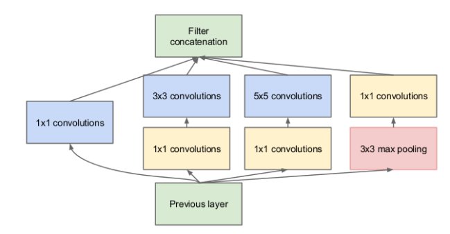
In 2015, the Inception architecture was proposed, the idea of which was as follows: instead of choosing the kernel size, let's take several options at once, use them all at the same time and concatenate the results. However, this significantly increases the number of operations that must be performed to calculate the activation of one layer, however the authors of the original article offering such trick: let before each convolution unit do convolution with the size of the kernel 1x1, reducing the dimension of the signal supplied to the svortkam entrance b of lshimi size of nuclei .
The resulting design below is the complete Inception module.
But what does this have to do to make our network more compact?
In 2016, François Chollet, the author and developer of the Keras framework, published an article that suggested going further and using the so-called extreme Inception module, also known as depthwise separable convolution.
Imagine that we took a standard convolution layer with 3x3 filters, the input of which is supplied with a dimensional tensor
  where
where  Is the width and height of the tensor, and
  - number of channels.
What makes such a layer? It collapses all the channels of the original signal simultaneously.different convolutions. At the output of such a layer, a dimension tensor is obtained .
.
Instead, let's take two steps sequentially:

Let's look at a specific example. Let us collapse the image with 16 channels with a convolutional layer with 32 filters. In total, this convolutional layer will have weights, since we will have
  3x3 roll.
How many weights will be in a similar depthwise separable convolution block? Firstly, we will have pointwise convolution weights. Secondly, we will have
 weights from depthwise convolution. In total, we get 800 weights, which is much less than a conventional convolutional layer.
An ordinary convolutional layer simultaneously processes both spatial information (correlation of neighboring points within one channel) and inter-channel information, since convolution is applied to all channels at once. The Xception architecture is based on the assumption that these two types of information can be processed sequentially without loss of network performance, and decomposes the usual convolution into pointwise convolution (which processes only inter-channel correlation) and spatial convolution (which processes only spatial correlation within a separate channel) .
Let's look at the real effect. For comparison, let's take two truly deep convolution network architectures - ResNet50 and InceptionResNetV2.
ResNet50 has 25 636 712 weights, and the pre-trained model in Keras weighs 99 MB. The accuracy achieved by this model on the ImageNet dataset is 75.9%.
InceptionResNetV2 has 55,873,736 learning parameters and weighs 215 MB, achieving an accuracy of 80.4%.
What about the Xception architecture? The network has 22,910,480 weights and weighs 88 MB. Moreover, the classification accuracy on ImageNet is 79%.
Thus, we get a network architecture that is superior to ResNet50 in accuracy and only slightly inferior to InceptionResNetV2, while significantly winning in size , and therefore in terms of required resources, both for training and for using this model.
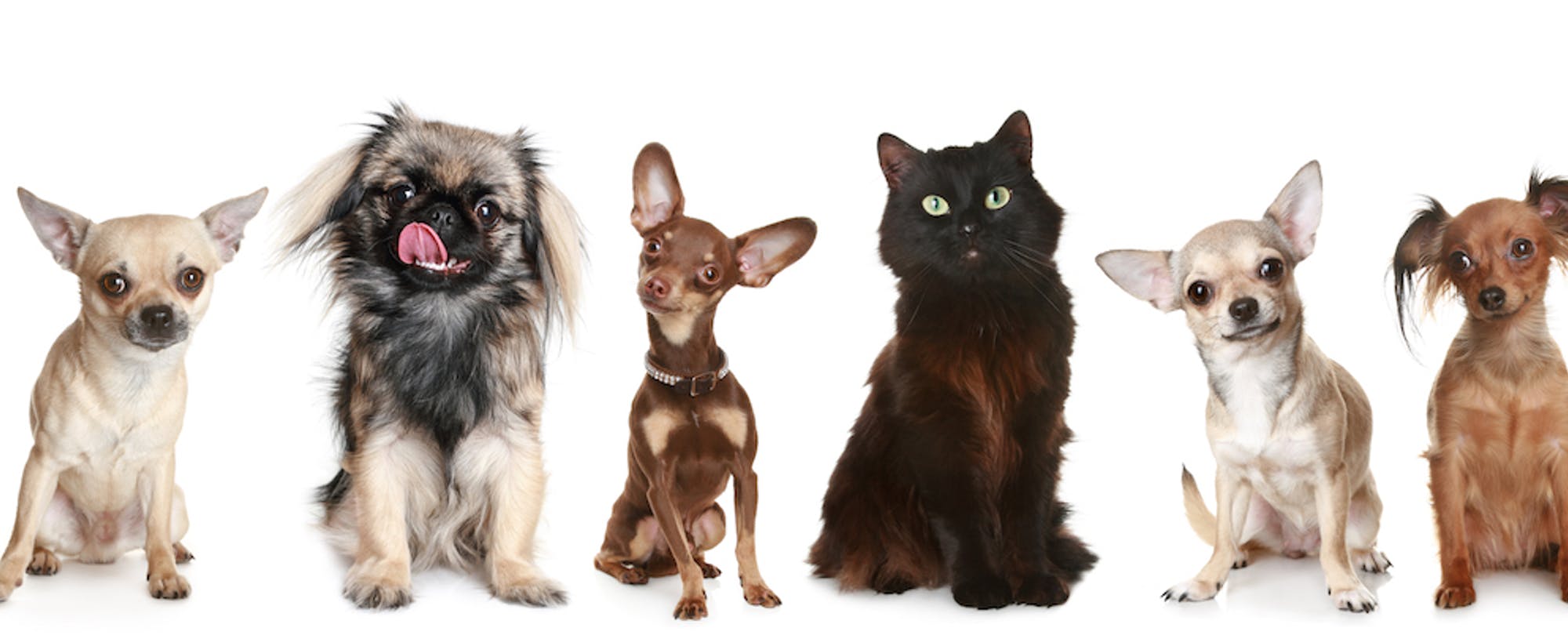
Let us examine with a short example how to apply this architecture to a real task. For these purposes, let's take the Dogs vs Cats dataset with Kaggle and in half an hour we will teach our network to distinguish cats from dogs.
We will divide the dataset into three parts: train (4000 images), validation (2000 images) and test (10000 images).
Since Francois Scholl, the author of the Xception architecture, is also the creator of Keras, he kindly provided the weights of this network trained on ImageNet in his framework, which we will use to reach the network for our task using transfer learning.
Load the weights from ImageNet into Xception, from which the last fully connected layers have been removed. Let's pass our dataset through this network to get the features that the convolutional network can extract from images (the so-called bottleneck features):
We will create a fully connected network and train it on the characteristics obtained from convolutional layers, using a specially deferred part of the initial data set for validation:
After this stage, which takes a couple of minutes on the GeForce GTX 1060, we get an accuracy of about 99.4% on the validation dataset.
Now we’ll try to retrain the network with augmentation of the input data by loading weights from ImageNet into convolutional layers, and weights into the fully connected layers that we just learned:
Having trained the network in this mode, in five more eras (about twenty minutes) we will achieve 99.5% accuracy on the validation dataset.
After checking the model on data that it has never seen and that were not used to configure hyperparameters (test dataset), we will see an accuracy of about 96.9%, which looks pretty acceptable.

The full code for this experiment can be found on GitHub .
In 2017, Google added pre- trained MobileNet architecture networks to TensorFlow , using principles similar to Xception, to make models even smaller. These models are suitable for performing computer vision tasks directly on mobile phones or IoT devices with extremely limited memory and a weak processor.
Thus, we imperceptibly approached the point in the history of computer science when you can write an application that determines whether a bird is shown in the photo in fifteen minutes, and this application will run directly on your smartphone.
If you want to know what it is and see how to use such a network in practice to learn how to distinguish cats from dogs, welcome to cat.
Module inception
Each time we add another layer to the convolution network, we need to make a strategic decision about its characteristics. What size convolution core should we use? 3x3? 5x5? Or maybe put max pooling?
In 2015, the Inception architecture was proposed, the idea of which was as follows: instead of choosing the kernel size, let's take several options at once, use them all at the same time and concatenate the results. However, this significantly increases the number of operations that must be performed to calculate the activation of one layer, however the authors of the original article offering such trick: let before each convolution unit do convolution with the size of the kernel 1x1, reducing the dimension of the signal supplied to the svortkam entrance b of lshimi size of nuclei .
The resulting design below is the complete Inception module.
But what does this have to do to make our network more compact?
In 2016, François Chollet, the author and developer of the Keras framework, published an article that suggested going further and using the so-called extreme Inception module, also known as depthwise separable convolution.
Depthwise separable convolution
Imagine that we took a standard convolution layer with
3x3 filters, the input of which is supplied with a dimensional tensor where Is the width and height of the tensor, and - number of channels. What makes such a layer? It collapses all the channels of the original signal simultaneously.
different convolutions. At the output of such a layer, a dimension tensor is obtained. Instead, let's take two steps sequentially:
- We collapse the original 1x1 tensor with a convolution, similar to what we did in the Inception block, getting the tensor
 . This operation is called pointwise convolution.
 - We will collapse each channel individually with a 3x3 convolution (in this case, the dimension will not change, since we do not collapse all the channels together, as in a conventional convolution layer). This operation is called depthwise spatial convolution.
A bit of tediousness about terminology.
In fact, usually when it comes to depthwise separable convolution, it is implied that they first convolve along the channels, and then 1x1 convolution, however, I give exactly the order of operations that is indicated in the original article. In general, according to the author, the order of these operations does not affect the final result.
Why does this make the network more compact?
Let's look at a specific example. Let us collapse the image with 16 channels with a convolutional layer with 32 filters. In total, this convolutional layer will have
weights, since we will have 3x3 roll. How many weights will be in a similar depthwise separable convolution block? Firstly, we will have
pointwise convolution weights. Secondly, we will haveweights from depthwise convolution. In total, we get 800 weights, which is much less than a conventional convolutional layer.Why does this even work?
An ordinary convolutional layer simultaneously processes both spatial information (correlation of neighboring points within one channel) and inter-channel information, since convolution is applied to all channels at once. The Xception architecture is based on the assumption that these two types of information can be processed sequentially without loss of network performance, and decomposes the usual convolution into pointwise convolution (which processes only inter-channel correlation) and spatial convolution (which processes only spatial correlation within a separate channel) .
Let's look at the real effect. For comparison, let's take two truly deep convolution network architectures - ResNet50 and InceptionResNetV2.
ResNet50 has 25 636 712 weights, and the pre-trained model in Keras weighs 99 MB. The accuracy achieved by this model on the ImageNet dataset is 75.9%.
InceptionResNetV2 has 55,873,736 learning parameters and weighs 215 MB, achieving an accuracy of 80.4%.
What about the Xception architecture? The network has 22,910,480 weights and weighs 88 MB. Moreover, the classification accuracy on ImageNet is 79%.
Thus, we get a network architecture that is superior to ResNet50 in accuracy and only slightly inferior to InceptionResNetV2, while significantly winning in size , and therefore in terms of required resources, both for training and for using this model.
Less words, more code.
Let us examine with a short example how to apply this architecture to a real task. For these purposes, let's take the Dogs vs Cats dataset with Kaggle and in half an hour we will teach our network to distinguish cats from dogs.
We will divide the dataset into three parts: train (4000 images), validation (2000 images) and test (10000 images).
Since Francois Scholl, the author of the Xception architecture, is also the creator of Keras, he kindly provided the weights of this network trained on ImageNet in his framework, which we will use to reach the network for our task using transfer learning.
Load the weights from ImageNet into Xception, from which the last fully connected layers have been removed. Let's pass our dataset through this network to get the features that the convolutional network can extract from images (the so-called bottleneck features):
input_tensor = Input(shape=(img_height,img_width,3))
base_model = xception.Xception(weights='imagenet',
                          include_top=False,
                          input_shape=(img_width, img_height, 3),
                          pooling='avg')
data_generator = image.ImageDataGenerator(rescale=1. / 255)
train_generator = data_generator.flow_from_directory(
    train_data_dir,
    target_size=(img_height, img_width),
    batch_size=batch_size,
    class_mode=None,
    shuffle=False)
bottleneck_features_train = base_model.predict_generator(
        train_generator,
        nb_train_samples // batch_size)
np.save(open('bottleneck_features_train.npy', 'wb'),
            bottleneck_features_train)
We will create a fully connected network and train it on the characteristics obtained from convolutional layers, using a specially deferred part of the initial data set for validation:
model = Sequential()
model.add(Dense(256, activation='relu', input_shape=base_model.output_shape[1:]))
model.add(Dropout(0.5))
model.add(Dense(128, activation='relu'))
model.add(Dropout(0.5))
model.add(Dense(1, activation='sigmoid'))
model.compile(optimizer=SGD(lr=0.01),
              loss='binary_crossentropy',
              metrics=['accuracy'])
checkpointer = ModelCheckpoint(filepath='top-weights.hdf5', verbose=1, save_best_only=True)
history = model.fit(train_data,
                    train_labels,
                    epochs=epochs,
                    batch_size=batch_size,
                    callbacks=[checkpointer],
                    validation_data=(validation_data, validation_labels))
After this stage, which takes a couple of minutes on the GeForce GTX 1060, we get an accuracy of about 99.4% on the validation dataset.
Now we’ll try to retrain the network with augmentation of the input data by loading weights from ImageNet into convolutional layers, and weights into the fully connected layers that we just learned:
input_tensor = Input(shape=(img_height,img_width,3))
base_model = xception.Xception(weights='imagenet',
                                            include_top=False,
                                            input_shape=(img_width, img_height, 3),
                                            pooling='avg')
top_model = Sequential()
top_model.add(Dense(256, activation='relu', input_shape=base_model.output_shape[1:]))
top_model.add(Dropout(0.5))
top_model.add(Dense(128, activation='relu'))
top_model.add(Dropout(0.5))
top_model.add(Dense(1, activation='sigmoid'))
top_model.load_weights('top-weights.hdf5')
model = Model(inputs=base_model.input, outputs=top_model(base_model.output))
model.compile(optimizer=SGD(lr=0.005, momentum=0.1, nesterov=True),
              loss='binary_crossentropy',
              metrics=['accuracy'])
Having trained the network in this mode, in five more eras (about twenty minutes) we will achieve 99.5% accuracy on the validation dataset.
After checking the model on data that it has never seen and that were not used to configure hyperparameters (test dataset), we will see an accuracy of about 96.9%, which looks pretty acceptable.
The full code for this experiment can be found on GitHub .
What's next?
In 2017, Google added pre- trained MobileNet architecture networks to TensorFlow , using principles similar to Xception, to make models even smaller. These models are suitable for performing computer vision tasks directly on mobile phones or IoT devices with extremely limited memory and a weak processor.
Thus, we imperceptibly approached the point in the history of computer science when you can write an application that determines whether a bird is shown in the photo in fifteen minutes, and this application will run directly on your smartphone.