January 10, 2018 at 00:46
Using the inverse Laplace transform to analyze the dynamic links of control systems
Hello!
Until now, the arsenal of tools of the high-level programming language Python did not include modules for the numerical conversion of the transfer functions of ACS elements from the frequency domain to the time domain.
Since the functions of the inverse Laplace transform are widely used in the analysis of dynamic measurement and control control systems, using Python for these purposes was very difficult, since it was necessary to use a less accurate inverse Fourier transform [1].
This problem is solved by the mpmath module of the Python free distribution library (licensed under BSD), designed to solve the problems of real and complex arithmetic with a floating point and a given accuracy.
Work on the module back in 2007 was started by Fredrik Johansson [2], and, thanks to the help of many project participants, mpmath has now acquired the capabilities of a serious mathematical package.
However, we will be interested only in the topic stated in the article, implemented using the one-step invertlaplace algorithm. As an example, we consider a comparison of the results of the inverse Laplace transform of the transfer function w (p) = 1 / (1 + p) ** 2 using invertlaplace with the known transition function h (t) = e ** - t of the specified transfer function:
Invertlaplace testing
from mpmath import *
import time
mp.dps = 15#число членов, используемых в приближении
mp.pretty = True
start = time.time()
def  run_invertlaplace(tt,fp,ft):
         for i in range(0,len(tt)):
               print('Значение тестовой функции : %s'%ft(tt[i]))
               print('Полученное значение функции : %s'%invertlaplace(fp,tt[i],method='talbot'))
               print(' Значение h(t) : %s. Абсолютная погрешность :%s.'%(ft(tt[i]), ft(tt[i])-invertlaplace(fp,tt[i],method='talbot')))
         stop = time.time()
         print ("Время, затраченное на обратное преобразование Лапласа: %s"%(stop-start))
tt = [0.001, 0.01, 0.1, 1, 10]#список значений отсчётов времени
fp = lambda p: 1/(p+1)**2#передаточная функция частоты для тестирования программы
ft = lambda t: t*exp(-t)# переходная функция времени для тестирования программы
run_invertlaplace(tt,fp,ft)
Test results:
Value of test function: 0.000999000499833375
Received value of function: 0.000999000499833375
h (t) value: 0.000999000499833375. Absolute error: 8.57923043561212e-20.
The value of the test function: 0.00990049833749168
The obtained value of the function: 0.00990049833749168
The value of h (t): 0.00990049833749168. Absolute error: 3.27007646698047e-19.
The value of the test function: 0.090483741803596
The obtained value of the function: 0.090483741803596
The value of h (t): 0.090483741803596. Absolute error: -1.75215800052168e-18.
The value of the test function: 0.367879441171442
The obtained value of the function: 0.367879441171442
H (t): 0.367879441171442 Absolute error: 1.2428864009344e-17.
The value of the test function: 0.000453999297624849
The obtained value of the function: 0.000453999297624849
The value of h (t): 0.000453999297624849. Absolute error: 4.04513489306658e-20.
The time spent on the inverse Laplace transform: 0.18808794021606445
The test example is limited in volume, but it also shows that the one-step invertlaplace algorithm has high accuracy and is not critical runtime for a limited number of time values.
In the considered example, the talbot method was used; the features of other methods can be found in the documentation [3].
However, it should be borne in mind that all numerical methods of the inverse Laplace transform require that their abscissa shift closer to the origin for large times. If the abscissa moves to the left of the rightmost coordinate in the Laplace region, the answer will be completely wrong.
Therefore, it is necessary to study the applicability of the numerical inverse Laplace transform for certain transfer functions and evaluate the error in comparison with another method, in this publication it is the inverse Fourier transform method.
1. The construction of the transition characteristics of the control object by its transfer function using invertlaplace
Suppose we have a water-water heat exchanger with a transfer function along the channel, the temperature of the heated water is the consumption of heating water. The Laplace transform of the output signal is the transfer function of the control object multiplied by 1 / p (unit perturbation in the consumption of heating water) taking into account the delay τ has the following form:

where: Ti are the time constants of the links; K is the static gear ratio; p ¬ Laplace operator.
Inverse Laplace transform of the transfer function (1)
# -*- coding: utf8 -*-
import numpy as np
import matplotlib.pyplot as plt
import matplotlib as mpl
from mpmath import *
mpl.rcParams['font.family'] = 'fantasy'
mpl.rcParams['font.fantasy'] = 'Comic Sans MS, Arial'
mp.dps = 5; mp.pretty = True
def  run_invertlaplace(tt,fp,tau):
      y=[]
      for i in np.arange(0,len(tt)):
               if tt[i]<=tau:
                        y.append(0)
               else:
                        y.append(invertlaplace(fp,tt[i],method='talbot'))
      return y
tau=5
tt = np.arange(0,100,0.05)
T1=5;T2=4;T3=4;K=1.5;tau=14
fp = lambda p: K*exp(-tau*p)/((T1*p+1)*(T2*p+1)*(T3*p+1)*p)
y=run_invertlaplace(tt,fp,tau)
plt.title('Переходная характеристика объекта управления \n, полученная через invertlaplace ')
plt.plot(tt,y,'r')
plt.grid(True)
plt.show()
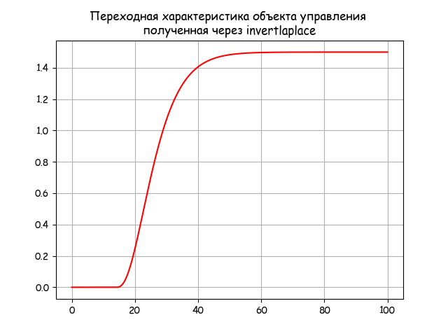
We obtain the transition characteristic of the object with delay and self-alignment:
2. The construction of the transient response of the PID controller by its transfer function using invertlaplace
The Laplace image of the transfer function of the PID controller has the form:

where: Td, Ti are the time constants of the differentiating and integrating links; Kp, Kd - static transmission coefficients of the proportional and differentiating links;
p is the Laplace operator.
Inverse Laplace transform of transfer function (2)
# -*- coding: utf8 -*-
import numpy as np
import matplotlib.pyplot as plt
import matplotlib as mpl
from mpmath import *
mpl.rcParams['font.family'] = 'fantasy'
mpl.rcParams['font.fantasy'] = 'Comic Sans MS, Arial'
mp.dps = 5; mp.pretty = True
tt = np.arange(0.01,20,0.05)
Kp=2;Ti=2;Kd=4;Td=0.5
fp = lambda p: (1+(Kd*Td*p)/(1+Td*p))*Kp*(1+1/(Ti*p))*(1/p)
y=[invertlaplace(fp,tt[i],method='talbot') for i in np.arange(0,len(tt))]
Kd=0
fp = lambda p: (1+(Kd*Td*p)/(1+Td*p))*Kp*(1+1/(Ti*p))*(1/p)
y1=[invertlaplace(fp,tt[i],method='talbot') for i in np.arange(0,len(tt))]
plt.title('Переходные характеристики регуляторов \n, полученные через invertlaplace ')
plt.plot(tt,y,'r', color='r',linewidth=2, label='ПИД-регулятор')
plt.plot(tt,y1, color='b', linewidth=2, label='ПИ-регулятор')
plt.grid(True)
plt.legend(loc='best')
plt.show()
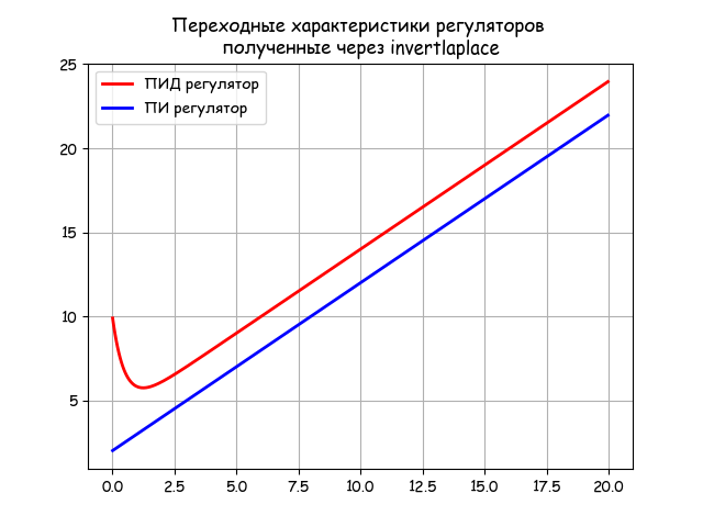
According to the listing, it is possible to obtain not only the transient response of the PID controller, but also the PI controller, taking Kd = 0:
3. Evaluation of the accuracy of the numerical inverse Laplace invertlaplace method as applied to typical ACS objects
Taking into account the caveats regarding the applicability of invertlaplace given at the beginning of the article, in the further presentation the applicability of the method to objects with delay and self-alignment, as well as to regulators, was proved.
The question of the accuracy of the numerical solution remains unclear. To clarify, we use the transfer function (2) and the following exact transformation to the transition function given in [1]:

Inverse transformation accuracy (2) using test function (3)
# -*- coding: utf8 -*-
import numpy as np
import matplotlib.pyplot as plt
import matplotlib as mpl
from mpmath import *
mpl.rcParams['font.family'] = 'fantasy'
mpl.rcParams['font.fantasy'] = 'Comic Sans MS, Arial'
mp.dps = 15; mp.pretty = True
tt = np.arange(0.01,20,0.01)
Kp=2;Ti=2;Kd=4;Td=0.5
fp = lambda p: (1+(Kd*Td*p)/(1+Td*p))*Kp*(1+1/(Ti*p))*(1/p)
ft = lambda t:(Kp/Ti)*(Ti+Kd*Td)+(Kp/Ti)*t+Kd*(Ti-Td)*exp(-t/Td)
y=np.array([invertlaplace(fp,tt[i],method='talbot') for i in np.arange(0,len(tt))])
y1=np.array([ft(tt[i]) for i in np.arange(0,len(tt))])
z=y-y1
plt.title('Оценка точности invertlaplace ')
plt.plot(tt,z,'r', color='r',linewidth=1, label='Разница между точным и численным решением')
plt.grid(True)
plt.legend(loc='best')
plt.show()
We get the following graph:
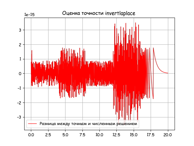
From the graph it can be seen that the error of the numerical method for the reduced class of transfer functions is negligible (3 * 10 ^ -15). In addition, the error of the numerical method can be controlled by setting the values mp.dps and the step tt [i + 1] -tt [i] (see listing).
4. A comparative assessment of the accuracy of the numerical method of the inverse Laplace transform invertlaplace and the numerical method of the inverse Fourier transform as applied to typical ACS objects
The transient response can be constructed on the basis of the inverse Fourier transform formula [1]:
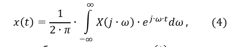
where X (j ∙ ω) is the Fourier image of the original x (t)
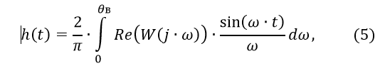
where Re (W (j ∙ ω)) is the real frequency characteristic of the control object.
As the upper limit of integration θv, the calculation takes the value of the frequency ωс at which the modulus Re (W (j ∙ ω)) decreases to a certain small value (for example, 0.05 * K) and does not exceed this value with a further increase in ω.
First, we define the upper limit of integration in relation (5). To do this, we use the transfer function (1), first getting rid of the unit impact, multiplying the right side by the operator p.
Plotting the function Re (W (j ∙ ω))
# -*- coding: utf8 -*-
import numpy as np
import matplotlib.pyplot as plt
import matplotlib as mpl
from mpmath import *
mpl.rcParams['font.family'] = 'fantasy'
mpl.rcParams['font.fantasy'] = 'Comic Sans MS, Arial'
ww= np.arange(0,0.6,0.005)
T1=25;T2=21;T3=12;K=0.37;tau=14
def invertfure(w):
         j=(-1)**0.5
         return ((K*np.exp(-tau*j*w)/((T1*j*w+1)*(T2*j*w+1)*(T3*j*w+1))).real)
z=[invertfure(w) for w in ww]
plt.title('Зависимость вещественной части передаточной функции \n  объекта управления Re(W(j*w)) от частоты ')
plt.plot(ww,z,'r')
plt.grid(True)
plt.show()
Graph:
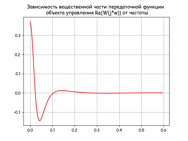
It can be seen from the graph that the upper limit of integration in relation (5) can be taken equal to 0.6, since with a further increase in the frequency, the real part of the transfer function of the control object retains a zero value.
Using (5), we obtain the transition characteristic of the control object by the inverse Fourier transform method:
Fourier transient response
# -*- coding: utf8 -*-
import numpy as np
import matplotlib.pyplot as plt
import matplotlib as mpl
from mpmath import *
mpl.rcParams['font.family'] = 'fantasy'
mpl.rcParams['font.fantasy'] = 'Comic Sans MS, Arial'
from scipy.integrate import quad
tt=np.arange(0,200,1)
T1=25;T2=21;T3=12;K=0.37;tau=14
def invertfure(w,t):
         j=(-1)**0.5
         return (2/np.pi)*((K*np.exp(-tau*j*w)/((T1*j*w+1)*(T2*j*w+1)*(T3*j*w+1))).real*(np.sin(w*t)/w))
z=[quad(lambda w: invertfure(w,t),0, 0.6)[0] for t in tt]
plt.title('Переходная характеристика объекта управления,   полученная \n методом обратного преобразования Фурье')
plt.plot(tt,z,'r')
plt.grid(True)
plt.show()
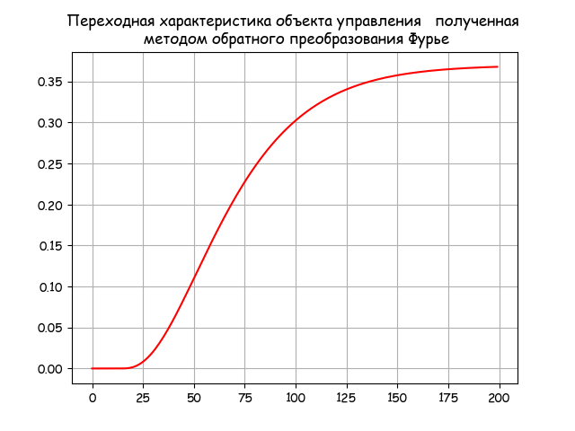
For a comparative assessment of the accuracy of the inverse Laplace and Fourier transform, we use the exact transformation of the transfer function (1) of the control object given in [1]:

From the exact transformation (6), we subtract in turn the inverse Laplace transform (1) and the inverse Fourier transform. To build a graph characterizing a comparison of the accuracy of both methods, we compile the following listing of the program:
Comparative analysis of the inverse Laplace and Fourier transform methods
# -*- coding: utf8 -*-
import numpy as np
from scipy.integrate import quad
import matplotlib.pyplot as plt
import matplotlib as mpl
mpl.rcParams['font.family'] = 'fantasy'
mpl.rcParams['font.fantasy'] = 'Comic Sans MS, Arial'
tt = np.arange(0,100,0.01)
T1=25;T2=21;T3=12;K=0.37;tau=14
def invertfure(w,t):
         j=(-1)**0.5
         return (2/np.pi)*((K*np.exp(-tau*j*w)/((T1*j*w+1)*(T2*j*w+1)*(T3*j*w+1))).real*(np.sin(w*t)/w))
z=np.array([quad(lambda w: invertfure(w,t),0, 0.6)[0] for t in tt])
def h(t):
         if t<=tau:
                  g=0
         else:
                  g=(-K*(T1**2)*np.exp((tau-t)/T1)/((T1-T3)*(T1-T2)))+(K*(T2**2)*np.exp((tau-t)/T2)/((T1-T2)*(T2-T3)))+(-K*(T3**2)*np.exp((tau-t)/T3)/((T1-T3)*(T2-T3)))+K
         return g
q=np.array([h(t) for t in tt])
from mpmath import *
mp.dps = 5; mp.pretty = True
def  run_invertlaplace(tt,fp,tau):
         y=[]
         for i in np.arange(0,len(tt)):
                  if tt[i]<=tau:
                           y.append(0)
                  else:
                           y.append(invertlaplace(fp,tt[i],method='talbot'))
         return y
fp = lambda p: K*exp(-tau*p)/((T1*p+1)*(T2*p+1)*(T3*p+1)*p)
y=np.array(run_invertlaplace(tt,fp,tau))
plt.title('Сравнительная оценка точности обратных \n Лапласа и Фурье преобразований ')
plt.plot(tt,q-y,'b',linewidth=2, label= 'Точное значение минус  обратное преобразование Лапласа')
plt.plot(tt,q-z,'r',linewidth=2, label='Точное значение минус обратное  преобразование Фурье')
plt.legend(loc='best')
plt.grid(True)
plt.show() 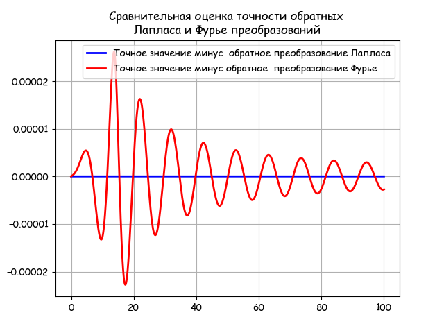
From the graph it follows that the numerical inverse Laplace transform is more stable than the Fourier transform and, in addition, it coincides with the exact solution.
conclusions
1. A comparative analysis of the numerical methods of the inverse Laplace and Fourier transform is carried out, the great accuracy and stability of the inverse Laplace transform is shown.
2. The possibilities of using the mpmath Python library for the inverse Laplace transform of the basic transfer functions of objects and elements of self-propelled guns are shown.