Bezier and Picasso Curves
- Transfer

Pablo Picasso in his studio on the background of the picture "Kitchen", a photograph of Herbert Liszt.
Artist and simplicity
One of my most favorite works by Pablo Picasso is his linear drawings. He depicted animals on some of them: an owl, a camel, a butterfly, etc. This work, entitled “The Dog,” hangs on my wall:
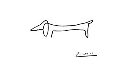
(You can go to the interactive demo in which we recreated the “Dog” using the mathematical calculations presented in the article)
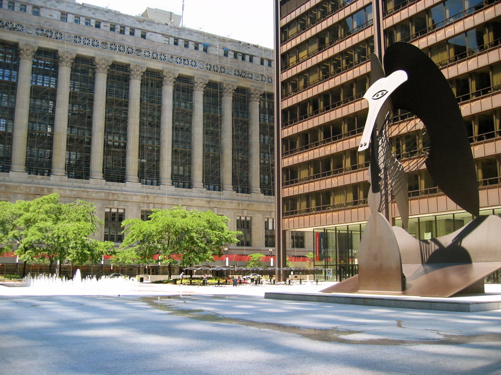
These drawings are extremely simple, but somehow they manage to deeply touch the viewer. They give the impression of simplicity of composition and implementation. A single hand movement and signature create a true masterpiece! The drawing at the same time seems both a careless improvisation and a precisely selected overture in a symphony of grace. In fact, we know that Picasso’s work process was deep. For example, in the years 1945-1946, Picasso created a series of eleven drawings (lithographs, more precisely), demonstrating his gradual progress in visualizing the bull. The former were more or less similar to realistic ones, but later on we see how the bull turns into its very essence, and the last figure consists of only a dozen lines. In the process of developing a series of drawings, we see a bull resembling some of Picasso's other works (number 9 reminds mesculpture at the Chicago Daley Center Plaza ). Here you can read more about a series of lithographs.

"The Bull" by Picasso. Photo taken by Jeremy Kuhn at the Art Institute in Chicago. Click on the image to enlarge it.
I will not pretend to be an experienced artist (I could not draw a bull, even if my life depended on it), but I can recognize the mathematical aspects of his paintings and write a damn good program. There is one obvious way to consider linear drawings in the style of Picasso as mathematical objects, and these are of course the Bezier curves. Let's start by studying the theory of Bezier curves, and then write a program to draw them. The mathematics used in it does not require any additional knowledge, except for the basics of algebra and polynomials, and I will try to go into complicated details as little as possible. We will learn a very simple algorithm for drawing Bezier curves, implement it in Javascript, and then recreate one of Picasso's linear drawings using several Bezier curves.
Bezier curves and parameterization
When someone asks to remember the “curves,” most people (possibly poisoned by teaching the basics of mathematics) either start to shake with fear, or draw part of the graph of the polynomial. Although these are perfectly correct and respected curves, they represent only a small part of the world of curves. We are especially interested in curves that are not part of the function graphs.

Three patterns.
For example, a pattern is a physical template used to (smoothly) draw smooth curves. Just connecting edges of any part of these curves, we usually can not get a graph of the function. Obviously, we need a more general idea of what curves are. The problem is that in different areas of mathematics, “curve” means different concepts. The curves that we will study called “Bezier curves” are a special case of polynomial plane curves with one parameter . It sounds too complicated, but actually it means that the whole curve can be defined by two polynomials: one for the values
 and second for values
  . Both polynomials have one variable, which we will call
 (defined on the set of real numbers).
 With an example, everything should become clearer. Let's pick two simple polynomials from
let's say  and
and  . If we want to find points on this curve, we simply select the valuesand substitute them in both equations. For example, substituting
 we get the point
  on the curve. Having all these values on the graph, we get a curve that is definitely not a graph of the function:
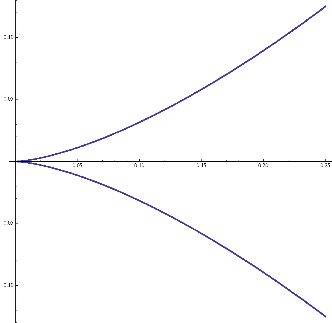
But it’s obvious that we can write any function with one variable
 in this parametric form: just choose
  and
and  . So, they are actually more general objects than ordinary functions (however, in this article we will only work with polynomials).
 We briefly repeat: a polynomial plane curve with one parameter is defined as a pair of polynomials
 from one variable . Sometimes, when we need to express the whole system in one equation, we can take the coefficients of the general degreesand write them as vectors and . Thanks to the example above
 we can rewrite it as
  .
. Here, the coefficients are points on the plane (the same as the vectors), and we select the function
 bold to emphasize that the output is a point. Learners of linear algebra can understand that pairs of polynomials form a linear space, and combine them as
 . But it will be more convenient for us to perceive points as coefficients of one polynomial.
 We also limit our attention to the consideration of one-parameter plane curves described by a polynomial for which the variable
allowed between zero and one. Such a restriction may seem strange, but in fact any finite one-parameter plane curve described by a polynomial can be written this way (we will not go into details of how this is implemented). For the sake of brevity, hereinafter I will call a one-parameter plane curve defined by a polynomial in whichis in the range from zero to one, just a “curve”. We can do very interesting things with these curves. For example, for any two points in the plane
 we can describe the line between them as a curve:
  . And in fact, with
 value
value  exactly equal
  at
at  exactly equal
  , and the equation is a linear polynomial for . Moreover (if you do not go into the details of matanalysis), the line
 runs at “unit speed” from before . In other words, we can perceive as describing the motion of a particle from in time and during
  the particle will go a quarter way, and during
  half way, etc. (An example of a straight line that does not have unit speed is, for example,
 .)
.) For a more general case, let's add a third point
 . We can describe the path through in , and he is "directed" by a point lying in the middle. This idea of a “guide” point is a bit abstract, but with respect to computing it is not more complicated. Instead of moving from one point to another at a constant speed, we want to move from one line to another at a constant speed. That is, we can name two curves that describe straight lines from
 and
and  crooked
  and
and  . Then the curve “guided” by a pointcan be written as a curve
Having completed all these multiplications, we get the formula

Point over time
 moves along a straight line between points
  and
and  that are also moving. So we get a curve that looks like this
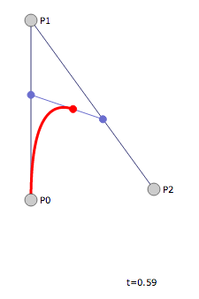
This screenshot is from Jason Davis, a terrific demo of data visualization consultant. He perfectly demonstrates the mathematical idea. In the demo, you can drag all three points to see how this affects the final curve. It’s worth playing with her for at least five minutes.
The whole idea of Bezier curves is to generalize this principle: having a list of points
 on the plane, we want to describe a curve that runs from the first to the last point, and "goes" between the other points. The Bezier curve is the realization of such a curve (a one-parameter plane curve defined by a polynomial), which becomes an inductive continuation of the one described above: we move at a unit speed from the Bezier curve given by the first
 list points to the last curve dots. In the simplest case, this is a straight line segment (or a single point, if you will). From a formal point of view,
 Definition: for a given set of points on a plane
we recursively define a Bezier curve of degree as
We will call
control points .
. Although the concept of moving at a unit speed between two lower-order Bezier curves is the essence of the matter (and allows us to approach the solution from a computational point of view), you can simply multiply all this (using the formula of binomial coefficients) and get the formula in explicit form. She will be next:

For example, a cubic Bezier curve with control points
 will have an equation
Higher order Bezier curves can be difficult to display geometrically. For example, the fifth degree Bezier curve (with six control points) is shown below.

Bezier curve of the fifth degree, illustration from Wikipedia.
The drawn additional line segments demonstrate the recursive nature of the curve. The simplest are green dots moving between control points. The blue dots move along the line segments between the green dots, the pink ones move between the blue dots, the orange between the pink ones, and finally, the red dot moves along the straight line between the orange dots.
Without the recursive structure of the problem (simply from observing the curve) it would be difficult to understand how all this can be calculated. But as we will see, the Bezier curve rendering algorithm is very natural.
Bezier curves as data and de Casteljo algorithm
Let's derive and implement the algorithm for rendering the Bezier curve on the screen, using only the ability to draw straight lines. For simplicity, we restrict ourselves to considering only Bezier curves of the third degree (cubic). And in fact, any Bezier curve by recursive definition can be written as a combination of cubic curves, and in practice cubic curves provide a balance between the efficiency of calculations and expressiveness. All the code in this post is written in Javascript and posted on the page of this blog on Github .
So, the cubic Bezier curve is represented in the program as a list of four points. For instance,
var curve = [[1,2], [5,5], [4,0], [9,3]];Most graphics libraries (including the standard HTML5 canvas ) have a graphics primitive that can display Bezier curves based on a four-point list. But suppose we do not have such a function. Suppose we can only draw straight lines. How can we draw an approximation of a Bezier curve? If such an algorithm exists (and it exists, and we will see this), then we can create such an accurate approximation that it will be visually indistinguishable from the true Bezier curve.
The most important property of Bezier curves that allows us to create such an algorithm is as follows:
Any cubic Bezier curve
from start to finish can be divided into two, which together will describe the same curve as . Let's see how to do it. Let be
will be a cubic bezier curve with control points , and suppose we want to divide it exactly in half. We will notice that the formula of the curve when substituted will take the form
Moreover, our recursive definition gives us a way to compute a point based on curves of a lesser degree. But when the calculations are performed at 1/2, their formulas are quite simple to write. The image looks like this:
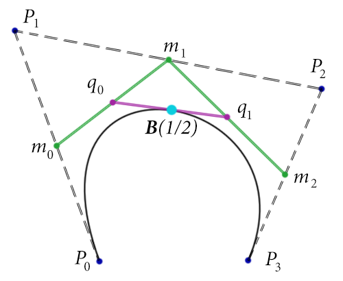
The green dots are first-degree curves, the pink dots are second-degree curves, and the blue dot is a cubic curve. We note that since each of the curves is calculated for
 , each of these points can be described as the midpoint of the points already known to us. therefore
 , etc.
 In fact, the division into two curves we need is precisely defined by these points. That is, half the curve is given
with breakpoints  while the "right" half
  has control points
  .
. How can we be sure that these are exactly the same Bezier curves? Well, these are just polynomials. We can test them for equality using intricate algebraic calculations. But it is worth noting that since
runs only halfway along  , then checking them for equality is similar to equating from
  , because the varies in the range from zero to one,
  varies in the range from zero to half. Similarly, we can compare
 from .
 Algebraic calculations are very confusing, but quite feasible. To prove this, I give a screencast of how I perform calculations proving the identity of two curves.
Now that we’ve checked everything, we have a good algorithm for dividing the cubic Bezier curve (or any Bezier curve) into two parts. In Javascript, it will look like this:
function subdivide(curve) {
   var firstMidpoints = midpoints(curve);
   var secondMidpoints = midpoints(firstMidpoints);
   var thirdMidpoints = midpoints(secondMidpoints);
   return [[curve[0], firstMidpoints[0], secondMidpoints[0], thirdMidpoints[0]],
          [thirdMidpoints[0], secondMidpoints[1], firstMidpoints[2], curve[3]]];
}
Here
curveis a list of four points, as described at the beginning of this section, and the output is a list of two curves with the correct control points. The function used is midpointsquite simple, and for completeness we will also add it here:function midpoints(pointList) {
var midpoint = function(p, q) {
return [(p[0] + q[0]) / 2.0, (p[1] + q[1]) / 2.0];
};
var midpointList = new Array(pointList.length - 1);
for (var i = 0; i < midpointList.length; i++) {
midpointList[i] = midpoint(pointList[i], pointList[i+1]);
}
return midpointList;
}It simply receives a list of points at the input and calculates their successive midpoints. That is a list of
 points turns into a list of points. As we saw, we need to call this function
 to calculate the segmentation of a Bezier curve of degree
  .
. As I explained earlier, we can continue to subdivide our curve again and again until each of the smaller parts becomes almost straight. That is, our function for drawing a Bezier curve will be as follows:
function drawCurve(curve, context) {
   if (isFlat(curve)) {
      drawSegments(curve, context);
   } else {
      var pieces = subdivide(curve);
      drawCurve(pieces[0], context);
      drawCurve(pieces[1], context);
   }
}
To put it in words, since our curve is not “flat,” we want to recursively subdivide and draw each part. If it is flat , then we can simply draw three straight line segments of the curve and logically assume that this will be a good approximation. The context variable used here is the canvas on which to draw; it needs to be transferred to the function
drawSegments, which simply draws a straight line on the canvas.Of course, this poses the obvious question: how can we determine that the Bezier curve is flat? There are many ways to do this. You can calculate the deviation angles (from the line) at each internal control point and add them. Or you can calculate the volume of the quadrilateral formed. However, calculating angles and volumes is usually not so convenient: it takes a lot of time to calculate angles, volumes have problems with stability, and stable algorithms are not very simple. We need a measurement for which simple arithmetic is sufficient and, possibly, checks for several logical conditions.
It turns out that such a dimension exists. It is initially attributed to Roger Wilcox, but it is quite simply displayed manually.
In essence, we want to measure the “flatness” of the cubic Bezier curve by calculating the distance from the real curve during
to where the curve should be duringif she is direct. Formally, having a given
with breakpoints , we can define a rectilinear cubic Bezier curve as a colossal sum
Nothing magical happens here. We just set a Bezier curve with control points
 . You need to take them as points that are on 0, 1/3, 2/3 and 1 share of the path from
 before
  in a straight line.
 Now we will set the function
 which will be the distance between two curves at the same time . Flatness value Is the maximum of the function in all respects . If the flatness value is below a certain tolerance level, then we will consider the curve flat.
 By adding a little algebra, we can simplify this expression. First, the meaning
, for which the distance is maximum, similar to the one with the maximum square, so we can avoid calculating the square root at the end and take this into account when choosing the flatness tolerance. Now let's write the difference as one polynomial. First, we can get rid of triples in
 and write the polynomial as
and therefore
 equals (when adding the coefficients of such terms

Out of brackets
 of both members and denoting
  ,
,  we get
Since the maximum of the product is the product of the maxima, we can limit the above value to the product of two maxima. The reason for this is that we can simply calculate the two maxima individually. It is easy to calculate the maximum without separation, but with this method we need fewer stages of calculations in the finished algorithm, and the visual result will be just as good.
Applying elementary calculations with a single variable, we obtain that the maximum value
 for
for  turns out to be equal
  . And the norm of a vector is just the sum of the squares of its components. If
 and
and  , then the norm presented above is
And note: for any real numbers
 value
value  exactly is a straight line from
  in
in  which is familiar to us. Maximum for everyone from zero to one will obviously be equal to the maximum of the end points . So the maximum of our distance function
 limited
And therefore, our flatness condition is that this restriction be less than a certain tolerance. We can safely factor 1/16 into this tolerance limit, and that will be enough to write the function.
function isFlat(curve) {
   var tol = 10; // всё, что меньше 50, выглядит довольно хорошо
   var ax = 3.0*curve[1][0] - 2.0*curve[0][0] - curve[3][0]; ax *= ax;
   var ay = 3.0*curve[1][1] - 2.0*curve[0][1] - curve[3][1]; ay *= ay;
   var bx = 3.0*curve[2][0] - curve[0][0] - 2.0*curve[3][0]; bx *= bx;
   var by = 3.0*curve[2][1] - curve[0][1] - 2.0*curve[3][1]; by *= by;
   return (Math.max(ax, bx) + Math.max(ay, by) <= tol);
}
There she is. We wrote a simple HTML page to access the canvas element and some helper functions for drawing line segments when the curve is flat enough, and presented the final result in this interactive demo (control points can be moved).
The image you see on this page (below) is my visualization of Picasso's “Dog”, drawn as a sequence of Bezier curves. I think that the resemblance is quite convincing.
Picasso's “Dog”, assembled from a sequence of nine Bezier curves.
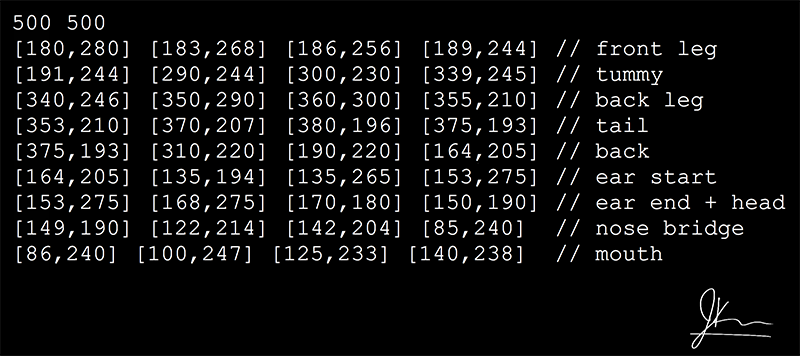
Although the drawing itself was not invented by us (and therefore cannot put our signature under it), we were able to present it as a sequence of Bezier curves. You can only call themart work. Here we reduced the view to a single file: the first line is the size of the canvas, and each subsequent line represents a cubic Bezier curve. Comments have been added for better readability.
The Dog, Jeremy Coon, 2013.
Standardization seems important to me, so we will define a new type of file ".bezier", which will have the format shown above:
int int
(int) curve
(int) curve
...
Here, the first two integers determine the size of the canvas, the first (optional) integer in each line defines the width of the line , and
curvehas the form[int,int] [int,int] ... [int,int]If there is no int at the beginning of the line, then the line is set to three pixels wide.
In general, a .bezier file can specify a curve with an arbitrary number of control points, however, the above code does not draw them in a general way. As an exercise, try writing a program that receives a .bezier file at the input, and creates a picture image at the output. To do this, you will need to expand the algorithm presented above so that it can draw arbitrary Bezier curves, cyclically performing calculations of midpoints and tracking those that turn out to be the final unit. Or you can write a program that receives a .bezier file at the input only with cubic Bezier curves, and produces an SVG file at the outputFigure (SVG only supports cubic Bezier curves). That is, the .bezier file is a simplification (less features) and an extension (Bezier curves of arbitrary degree) of the SVG file.
We did not delve into the theory of Bezier curves as much as we could. If you want to study the topic more deeply (and using matanalysis), then see this long introductory course . It contains almost everything you need to know about Bezier curves, as well as interactive demos written in Processing.
Art of low complexity
What we have done with Picasso's “Dog” has some philosophical significance. Earlier in this blog, we explored the idea of art of low complexity , and here it is fully applicable. The main idea is that “beautiful” art has a short description; if more formally, then the “complexity” of the object (presented in the text) is the length of the shortest program that produces this object in the absence of input data. You can read more about this in our introduction to Kolmogorov complexity . The fact that we can describe Picasso’s linear drawings with a small number of Bezier curves (and a relatively short program that produces Bezier curves) should be a deep statement about the beauty of art itself. Obviously, this view is very subjective, but it has its ownsupporters .
Today, there is interest in computer-generated art. For example, in these recent programming competitions (Dutch article), participants were given the task of generating a drawing reminiscent of the work of Pete Mondrian . The idea was that the more elegant the algorithm, the higher its score. To generate the works of Mondrian, the winner used MD5 hashes, and there are many other impressive examples (the gallery of finished works is presented at the link above).
In a previous post about art of low complexity, we explored the possibility of representing all images in a coordinate system that uses circles with a filled inner space. But it is obvious that in such a coordinate system it is impossible to imagine a “Dog” with very low complexity. It seems that Bezier curves are much more natural coordinate systems. Minor improvements, including line lengths and small distortions, do not affect the final complexity. A cubic Bezier curve can be described by any set of four points, and for more “intricate” descriptions (with increased complexity), a larger number of points is required. Bezier curves can be scaled arbitrarily, and this will not significantly change the complexity of the curve (even though that scaling by many orders of magnitude will add an increase in complexity with a logarithmic factor, it is quite small). Curves with a large line width are slightly more complicated than with a small width, and more curves are needed to represent many small sharp bends than for long and smooth arcs.
The disadvantage is the difficulty of representing in the form of a Bezier curve of a circle. In fact, it’s impossible to do it for sure . Despite the simplicity of this object (it is even given as the only polynomial, albeit with two variables), the best thing to do with it is to approximate it. The same applies to ellipses. There are actually ways around this problem (the concept of rational Bezier curves , which are partial polynomials), but they add inherent complexity to the rendering algorithm, and approximations using ordinary Beziers curves look pretty good.
So, we will define the complexity of the picture as the number of bits in the form of a .bezier file (comments are not taken into account in the calculations).
The real reward that we are still exploring will be finding a way to automatically generate art. That is, the implementation of one of two possibilities:
- After asking something like a random seed, write a program that creates a pseudo-random linear pattern.
- Having set the pattern, create a .bezier image that faithfully reproduces the pattern as a linear pattern.
We will try to explore these possibilities in a subsequent post. This may require some local search algorithms, genetic algorithms, or other methods.