Excel filters as a refactoring tool
- Tutorial
There was a need to conduct data processing. Due to the presence of discontinuous parts of the table, processing requires additional manual manipulations, and also complicates the automation of statistics processing. It was decided to remove the delimiters containing the date of test completion and a brief summary. There is a problem that for each result this date should be indicated, as well as the receiving testologist. The problem is solved by adding a column with this information. The following explains one of the simplest methods for making such information without applying programming knowledge.
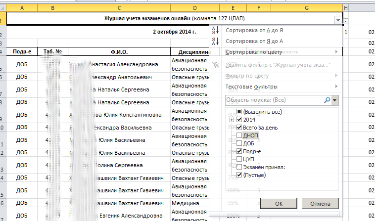
The source document is shown in the figure below.

Although the example indicates the work only in a sheet with the name “October”, the final version involves the merger of all such tables, and this is two dozen sheets. Therefore, manual copying from the date headers opposite each of the test results is time-consuming.
The first step is to select the entire document ([Ctrl] + A, [Ctrl] + A) and apply the filter. Because date headers are entered in the combined cells that begin with the first column, then the filter for these cells will be in the first filter. For the time being, we are only interested in dates, so we select only dates in the filter list.

The filter worked wonderfully and displayed only lines containing the dates the tests were passed.

Opposite the first date we put some kind of symbol or number, which, in essence, will be a flag that the cell on the left contains the date. Copy this cell and, having selected the entire column, paste the value.

Now we’ll make a condition in the cell to the right of our flag, which allows you to display a particular date. The formula for the condition is simple: if there is a unity in the cell on the left, then we take the date value to the left; if there is no one, then we take the date that is in the previous line.

Do not forget to select the “Date” cell format for the entire column.
We cancel the filter so that all lines are displayed, select the cell with our formula and drag its corner to the very bottom of the sheet - on all lines.

As a result, a date will appear opposite each line. If the title changes the date, then in the new column the date will change to a new one.

In the future, you will need to delete unnecessary lines, but the date column contains formulas with links, so you need to get rid of the links, leaving only the text. It is enough to select the entire column, copy it and paste with the parameter “only values”.

The next step is to remove the extra lines. In this example, each student has a note from which department he is, we will use this as a sign that this is a record of the test result. In the first filter, we’ll hide all the records according to the test results, as well as the record of the testologist conducting the test (this information is still useful to us).
We don’t need the displayed rows, except for the row with column headers.

Select all the rows except the one containing the column names and delete them.

Because Since we highlighted the filter line, the filtering of elements will be automatically disabled.

Turn on the filter again and select only the records about the tester.

To mark each entry next to who took the test, you can use the same method that was used to set the dates. But there is one difference - the dates in the delimiting headers were in front of the list of test takers, but the indication of who took the test is after the list.
We put the units in front of each surname of the testologist, but let's start writing the formula from the end. The condition is not much different - if the unit is in the cell, then we will also display the surname, and if not, we will display the surname from the bottom line (for the dates, select the cell above).

Turn off the filter and stretch the formula to the very top.

The names of the examiners are arranged for each entry.

In the same way as for dates, delete the link information by copying the column and pasting only the values.

We put the filter on the last names back and delete the extra lines.

Let's remove the filter and the “for ones” column, give names to the new columns and put a new filter. Now we have a table containing the data in a form suitable for processing.

The resulting table allows you to apply filters by date, allows you to calculate the average values and their number by a combination of filter and selection. For example, we select a filter for a specific week and select the column with the percentage of test completion - in the lower right, Excel displays the number of elements and their average value. Also, this table can be used as a data source for other applications, without worrying about filtering headers between records and other emerging issues.
The source document is shown in the figure below.
Although the example indicates the work only in a sheet with the name “October”, the final version involves the merger of all such tables, and this is two dozen sheets. Therefore, manual copying from the date headers opposite each of the test results is time-consuming.
The first step is to select the entire document ([Ctrl] + A, [Ctrl] + A) and apply the filter. Because date headers are entered in the combined cells that begin with the first column, then the filter for these cells will be in the first filter. For the time being, we are only interested in dates, so we select only dates in the filter list.
The filter worked wonderfully and displayed only lines containing the dates the tests were passed.
Opposite the first date we put some kind of symbol or number, which, in essence, will be a flag that the cell on the left contains the date. Copy this cell and, having selected the entire column, paste the value.
Now we’ll make a condition in the cell to the right of our flag, which allows you to display a particular date. The formula for the condition is simple: if there is a unity in the cell on the left, then we take the date value to the left; if there is no one, then we take the date that is in the previous line.
Do not forget to select the “Date” cell format for the entire column.
We cancel the filter so that all lines are displayed, select the cell with our formula and drag its corner to the very bottom of the sheet - on all lines.
As a result, a date will appear opposite each line. If the title changes the date, then in the new column the date will change to a new one.
In the future, you will need to delete unnecessary lines, but the date column contains formulas with links, so you need to get rid of the links, leaving only the text. It is enough to select the entire column, copy it and paste with the parameter “only values”.
The next step is to remove the extra lines. In this example, each student has a note from which department he is, we will use this as a sign that this is a record of the test result. In the first filter, we’ll hide all the records according to the test results, as well as the record of the testologist conducting the test (this information is still useful to us).
We don’t need the displayed rows, except for the row with column headers.
Select all the rows except the one containing the column names and delete them.
Because Since we highlighted the filter line, the filtering of elements will be automatically disabled.
Turn on the filter again and select only the records about the tester.
To mark each entry next to who took the test, you can use the same method that was used to set the dates. But there is one difference - the dates in the delimiting headers were in front of the list of test takers, but the indication of who took the test is after the list.
We put the units in front of each surname of the testologist, but let's start writing the formula from the end. The condition is not much different - if the unit is in the cell, then we will also display the surname, and if not, we will display the surname from the bottom line (for the dates, select the cell above).
Turn off the filter and stretch the formula to the very top.
The names of the examiners are arranged for each entry.
In the same way as for dates, delete the link information by copying the column and pasting only the values.
We put the filter on the last names back and delete the extra lines.
Let's remove the filter and the “for ones” column, give names to the new columns and put a new filter. Now we have a table containing the data in a form suitable for processing.
The resulting table allows you to apply filters by date, allows you to calculate the average values and their number by a combination of filter and selection. For example, we select a filter for a specific week and select the column with the percentage of test completion - in the lower right, Excel displays the number of elements and their average value. Also, this table can be used as a data source for other applications, without worrying about filtering headers between records and other emerging issues.