About fractals, martingales and random integrals. Part one

In my opinion, stochastic calculus is one of those magnificent sections of higher mathematics (along with topology and complex analysis), where formulas meet with poetry; this is the place where they find beauty, the place where the scope for artistic creation begins. Many of those who read the article Wiener Chaos or Another way to flip a coin , even if they understood a little, still managed to appreciate the magnificence of this theory. Today we will continue our mathematical journey, we will plunge into the world of random processes, non-trivial integration, financial mathematics, and even a little touch on functional programming. I warn you, keep your gyrus ready, as we have a serious conversation.


By the way, if you are interested in reading in a separate article, then suddenly it turned out that

$$

I added a poll below where you can leave your vote.

The hidden threat of fractals

Imagine some simple function $$ at some interval $$. Presented? In standard mathematical analysis, we are used to the fact that if the size of this interval is reduced for a sufficiently long time, then the function given to us starts to behave quite smoothly, and we can approximate it by a straight line, in extreme cases, a parabola. All thanks to the function decomposition theorem formulated by the English scientist Brooke Taylor in 1715:

$$

This theorem is skillfully handled by modern mathematicians and engineers, approximating everything in a row for their numerical calculations. But on fractals such a scheme fails.

By the time Benoit Mandelbrot came up with the very concept of “fractals”, they had not let many world scientists sleep for a hundred years. One of the first to whom fractals tarnished the reputation was Andre-Marie Ampère. In 1806, the scientist put forward a rather convincing "proof" that any function can be divided into intervals of continuous functions, and those, in turn, due to continuity, must have a derivative. And many of his contemporaries mathematicians agreed with him. In general, Ampère cannot be blamed for this seemingly rather crude mistake. The mathematicians of the beginning of the 19th century had a rather vague definition of such now basic concepts of mathematical analysis as continuity and differentiability, and, as a result, could be very mistaken in their proofs. Not even an exception were such eminent scientists as Gauss, Fourier, Cauchy, Legendre, Galois,

Nevertheless, in 1872, Karl Weierstrass refuted the hypothesis of the existence of derivatives of continuous functions by presenting the world's first fractal monster, which is continuous everywhere and nowhere differentiable.

Here, for example, how a similar function is set:

$$

The Brownian movement also possesses the same property (by the way, for some reason, it’s not Br but Unovsky, the surname is British, nevertheless). Brownian motion is a continuous random process$$such that all its increments are independent and have a normal distribution:

$$

The trajectories of the Brownian motion are fractal functions, they are continuous everywhere and non-smooth. But if the Weierstrass function was just a counterexample, even if it was one of the brightest mathematical analysis in the entire history, the Brownian movement promised to become the foundation of stochastic theory, and somehow it was necessary to learn how to work with it.

Endless variation of Brownian motion

Let's imagine a function again $$ on the interval $$ and divide this interval into many of $$ disjoint subintervals:

$$

We don't care how the points are distributed $$, dividing this interval, the size of the maximum step is much more interesting: $$ We will call the quantity

$$

a variation of the (first kind) function$$(also called common variation). If$$then we will say that $$has a finite variation. For example, a variation of a sufficiently “smooth” function

will be the ultimate. In which case are we not so sure? Well, for example, the function will not have final variation

$$

returning $$ for all rational $$ and $$for all irrational. Similar logic can be extended to random functions. Let it$$Is a random process. Variation for it is set in the same way:

$$

The only difference is that the variation will also become random (parameter $$ can be omitted for convenience, but he is here hinting that the variation from a random process is a mapping from the space of random events $$ in $$)

Here's what a fairly simple implementation of variation on Haskell will look like:

-- | 'totalVariation' calculates total variation of the sample process X(t)
totalVariation :: [Double] -- process trajectory X(t)
               -> Double   -- V(X(t))
totalVariation x@(_:tx) = sum $ zipWith (\x xm1 -> abs $ x - xm1) tx x

Where in the real world do random processes occur? One of the most famous examples today is financial markets, namely the movement of prices for currencies, stocks, options and various securities. Let it$$Is the value of an Apple share. At some point in time you decide to buy$$ stock price $$, and after a certain period of time the price changed and became equal to $$. As a result you$$ net profit / loss, where $$. You decided to buy / sell part of the shares and now you are holding$$valuable papers. After some time, your income / loss will amount to$$, etc. In the end, you will earn / lose

$$

Everything is quite simple, but here's the catch: the process of changing the price of a share can move very quickly, like our process of buying / selling it (the so-called High Frequency Trading). I would like to expand these calculations to continuous processes and present our income in the form of an integral like$$The problem is that we do not yet know how to take integrals over random processes and their trajectories. But we remember by what principle the standard Lebesgue integral (-Stieltjes) is determined. Usually, you first need to set the appropriate measure. Take a non-decreasing process$$, for simplicity, starting from scratch: $$, and a non-negative measure corresponding to its increments

$$

If the function $$ limited and measurable (recall the functional analysis), we can determine the integral for it on the interval $$ as

$$

For the general case, if the trajectories of a random process are not monotonic, we can divide it into two non-decreasing processes: $$ and then we define the Lebesgue integral as

$$

A necessary condition for the existence of such an integral is the existence $$. Indeed, if our process consists of the difference of two non-decreasing processes, then it has a finite variation (in the second line we used the triangle inequality):

$$

By the way, this condition also works in the opposite direction: if we have a process $$ with finite variation, then we can determine $$ and $$. Monotony and equality$$easy to prove.

Now we can easily integrate something. Take the trajectory of some continuous random process and call it$$. Using the Lagrange mean theorem, we can show that for a continuous function$$ the variation will be equal $$. If this integral exists, then under the conditions of boundedness and measurability mentioned above$$ we can count

$$

This is really easy. What about fractals, trajectories like the Weierstrass monster? After all, for them it does not exist$$.



So the question is: is it possible to take the integral in the sense of Lebesgue from the Brownian motion? We calculate the variation, and if it is finite, then we should not have any problems. Let's go from the side of the so-called quadratic variation :

$$

What do you think this limit is equal to? We consider a random variable$$ and show that its dispersion is zero:

$$

Where

$$

standard normally distributed value. In particular, since all$$ are independent and have a chi-square distribution with degree 1, it is easy to calculate that

$$

Consequently,

$$

In other words,

$$

Remember this formula! It is the foundation of stochastic analysis, a peculiar local analogue of the central limit theorem, and all other theorems explicitly and implicitly revolve around it.

Note that$$However, the methods for calculating these two quantities are completely different. The variance of the Brownian motion is considered to be the averaging of all its trajectories, given their probabilities. The quadratic variation is taken from one single random trajectory along which the movement occurred, and the probabilities do not play a role here. While the variance can only be calculated theoretically, since it requires averaging of all implementations, the quadratic implementation can be calculated explicitly (with a sufficient data discretization). The above formula is interesting in particular in that, by definition, a quadratic variation, like a variation of the first kind$$is a random variable. However, the feature of Brownian motion is that its quadratic variation degenerates and assumes only one single value, corresponding to the length of the interval, regardless of which trajectory the movement took.

Let's write a code that considers the quadratic variation of the implementation of a random process$$:

-- | 'quadraticVariation' calculates quadratic variation of the sample process X(t)
quadraticVariation :: [Double] -- process trajectory X(t)
                   -> Double   -- [X(t)]
quadraticVariation x@(_:tx) = sum $ zipWith (\x xm1 -> (x - xm1) ^ 2) tx x

So, now we are ready to return to calculating the variation of interest to us $$. We found out that

$$

That is, it is a nonzero, but not infinite value. On the other hand, it is bounded above by the maximum step of the broken$$:

$$

We know that Brownian motion is a continuous process, which means

$$

However, $$ And as a consequence,

$$

Oh yeah ...

Ito Integral or New Hope

In 1827, the English botanist Robert Brown, observing pollen grains in water through a microscope, noticed that the particles inside their cavity move in a certain way; however, he was then unable to identify the mechanisms that caused this movement. In 1905, Albert Einstein published an article explaining in detail how the movement observed by Brown was the result of pollen moving by individual water molecules. In 1923, the child prodigy and “father of cybernetics,” Norbert Wiener, wrote an article on differentiable spaces, where he approached this movement from the side of mathematics, determined probability measures in the space of trajectories and, using the concept of Lebesgue integrals, laid the foundation for stochastic analysis. Since then, in the mathematical community, the Brownian motion is also called the Wiener process.

In 1938, a graduate of Tokyo University Kiyoshi Ito begins to work in the Bureau of Statistics, where in his free time he gets acquainted with the work of the founder of modern probability theory, Andrei Kolmogorov, and the French scientist Paul Levy, who was studying at that time various properties of the Brownian movement. He tries to combine Levy’s intuitive visions with Kolmogorov’s exact logic, and in 1942 he wrote “On Stochastic Processes and Infinitely Divisible Distribution Laws,” in which he reconstructs from scratch the concept of stochastic integrals and the associated theory of stochastic differential equations describing the motions caused by random events.

Ito integral for simple processes

Ito developed a fairly simple way to build an integral. First, we define the Ito integral for a simple piecewise constant process$$and then we extend this concept to more complex integrands. So let us have a split again$$. We believe that the values$$ constant at each interval $$

Imagine that $$ Is the value of a financial instrument at the time $$(Brownian movement can take negative values, so this is not a good model for price movement, but now we will ignore it). Let also$$ - these are trading days (hours / seconds, it doesn’t matter), and $$- this is our position (the number of financial instruments on hand). We believe that$$ depends only on information known at the time $$. By information, I mean the trajectory of the Brownian motion up to this point in time. Then our income will be:

$$

Process $$called ito integral for a simple process$$ and we will write it in the form

$$

This integral has several interesting properties. The first and rather obvious: at the initial moment, its mathematical expectation at any point is zero:

$$

Moreover, the Ito integral is a martingale, but more on that later.

The calculation of the second moment / variance already requires additional calculations. Let it$$ for $$ and $$. Then we can rewrite the Ito integral in the form

$$

Taking advantage of the fact that $$ and the fact that $$ and $$ independent for $$ we can calculate

$$

Equality

$$

called Ito isometry .

And finally, a quadratic variation. Let's first calculate the variation on each interval$$where the values $$are constant, and then we put them all together. Take a partitioning interval$$ and consider

$$

Similarly, the quadratic variation for the interval is considered $$. Summing up all these pieces, we get

$$

Now we can clearly see the difference between dispersion and variation. If the process$$is determinate then they match. But if we decide to change our strategy depending on the trajectory along which the Brownian motion has passed, then the variation will begin to change, while the variance is always equal to a certain value.

Ito integral for complex processes

Now we are ready to expand the concept of the Ito integral to more complex processes. Let us have a function$$, which can continuously change over time and even have gaps. The only assumptions we want to keep are the quadratic process integrability:

$$

and adaptability , i.e. at the moment$$when we know the meaning $$we should already know the meaning $$. In the real world, we cannot first find out the value of shares for tomorrow, and then invest in them.

In order to determine$$ we approximate $$simple processes. The graph below shows how this can be done.


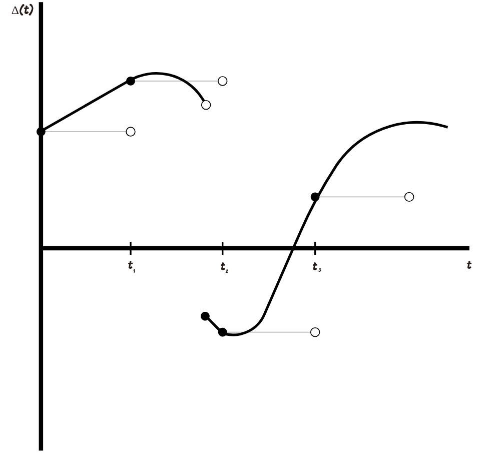
The approximation is as follows: we choose a partition $$, then create a simple process whose values ​​are equal $$ for everybody $$ and do not change on the segment $$. The smaller the maximum step of our partition becomes, the closer the approximating simple process becomes to our integrand.

In general, it is possible to choose a sequence of simple processes$$such that it will converge to $$. By convergence we mean

$$

For every process $$ Ito integral is already defined and we define the Ito integral for a continuously changing process as a limit:

$$

The Ito integral in the general case has the following properties:

• Its trajectories are continuous
• It is adapted. It is logical, because at every moment of time we must know our value of income.
• It is linear: $$
• He is a martingale, but more on that near the end of the article.
• Iso Itometry saved: $$.
• Its quadratic variation: $$

A small remark: for those who want to study the construction of the Ito integral in more detail or are generally interested in financial mathematics, I highly recommend Steven Shreve's book “Stochastic Calculus for Finance. Volume II ".

Let's go?

For the following reasoning, we will denote the Itô integral in a slightly different form:

$$

for some $$. Thus, we prepare ourselves for the idea that the Itô integral is a map acting from the space of quadratically integrable functions$$into the probability space of random processes. So for example, you can go from the old notation to the new one:

$$

In the previous article, we implemented the Gaussian process:$$. We know that a Gaussian process is a mapping from a Hilbert space to a probability one, which is essentially a generalized case of the Ito integral, a mapping from a space of functions to a space of random processes. Really,

data L2Map = L2Map {norm_l2 :: Double -> Double}
type ItoIntegral = Seed         -- ω, random state
                -> Int          -- n, sample size
                -> Double       -- T, end of the time interval
                -> L2Map        -- h, L2-function
                -> [Double]     -- list of values sampled from Ito integral
-- | 'itoIntegral'' trajectory of Ito integral on the time interval [0, T]
itoIntegral' :: ItoIntegral
itoIntegral' seed n endT h = 0 : (toList $ gp !! 0)
  where gp = gaussianProcess seed 1 (n-1) (\(i, j) -> norm_l2 h $ fromIntegral (min i j + 1) * t)
        t = endT / fromIntegral n

The itoIntegral function ' takes seed as an input - a parameter for a random generator, n - the dimension of the output vector, endT - parameter$$and the function h from the L2Map class, for which the norm_l2 function is defined , which returns the norm of the integrand:$$. At the output, itoIntegral issues an implementation of the Ito integral on the interval$$with a sampling rate corresponding to parameter n . Naturally, a similar way of implementing the Ito integral is in some sense an overkill, but it allows you to tune in to the functional thinking that is so necessary for further reasoning. We will write a faster implementation that does not require work with giant matrices.

-- | 'mapOverInterval' map function f over the interval [0, T]
mapOverInterval :: (Fractional a) => Int      -- n, size of the output list
                                  -> a        -- T, end of the time interval
                                  -> (a -> b) -- f, function that maps from fractional numbers to some abstract space
                                  -> [b]      -- list of values f(t), t \in [0, T]
mapOverInterval n endT fn = [fn $ (endT * fromIntegral i) / fromIntegral (n - 1) | i <- [0..(n-1)]]
-- | 'itoIntegral' faster implementation of itoIntegral' function
itoIntegral :: ItoIntegral
itoIntegral seed 0 _    _ = []
itoIntegral seed n endT h = scanl (+) 0 increments
  where increments = toList $ (sigmas hnorms) * gaussianVector
        gaussianVector = flatten $ gaussianSample seed (n-1) (vector [0]) (H.sym $ matrix 1 [1])
        sigmas s@(_:ts) = fromList $ zipWith (\x y -> sqrt(x-y)) ts s
        hnorms = mapOverInterval n endT $ norm_l2 h

Now, using this function, we can implement, for example, the ordinary Brownian motion: $$. The function h is a function, in which the norm norm_l2 will$$, identical function.

l2_1 = L2Map {norm_l2 = id}
-- | 'brownianMotion' trajectory of Brownian motion a.k.a. Wiener process on the time interval [0, T]
brownianMotion :: Seed     -- ω, random state
               -> Int      -- n, sample size
               -> Double   -- T, end of the time interval
               -> [Double] -- list of values sampled from Brownian motion
brownianMotion seed n endT = itoIntegral seed n endT l2_1

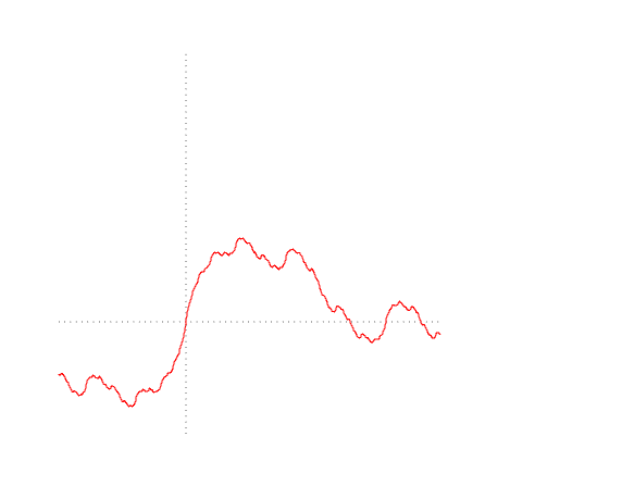
Let's try to draw different options for the trajectories of Brownian motion

import Graphics.Plot
let endT = 1
let n = 500
let b1 = brownianMotion 1 n endT
let b2 = brownianMotion 2 n endT
let b3 = brownianMotion 3 n endT
mplot [linspace n (0, lastT), b1, b2, b3]

It's time to double-check our previous calculations. Let's calculate the variation of the Brownian motion trajectory on the interval$$.

Prelude> totalVariation (brownianMotion 1 100 1)
8.167687948236862
Prelude> totalVariation (brownianMotion 1 10000 1)
80.5450335433388
Prelude> totalVariation (brownianMotion 1 1000000 1)
798.2689137110999

We can observe that with increasing accuracy, the variation takes on larger and larger values, while the quadratic variation tends to $$:

Prelude> quadraticVariation (brownianMotion 1 100 1)
0.9984487348804609
Prelude> quadraticVariation (brownianMotion 1 10000 1)
1.0136583395467458
Prelude> quadraticVariation (brownianMotion 1 1000000 1)
1.0010717246843375

Try running the calculation of variations for arbitrary Ito integrals to make sure that $$ regardless of the trajectory of movement.

Martingales

There is such a class of random processes - martingales . In order to$$ was martingale, three conditions must be met:

• It is adapted
• $$ almost everywhere of course:

  $$

• Conditional mathematical expectation of the future value $$ equals its last known value:

  $$

Brownian movement - martingale. The fulfillment of the first condition is obvious, the fulfillment of the second condition follows from the properties of the normal distribution. The third condition is also easily verified:

$$

The Ito integral is also a martingale (let us leave the proof as an exercise). What does this tell us? Let us return to financial mathematics and imagine that the value of the stocks we have chosen is Brownian motion (the assumption is rather naive, but still imagine), and$$- this is our strategy, the number of shares in our portfolio. Process$$ may be random: we do not always know very much in advance how many stocks we want to keep, we will proceed from the price movement $$. But the main thing is that this process be adapted, that is, at the time$$we know exactly how many stocks we have. We cannot return to the past and change this meaning. So, since the Ito integral is a martingale, it doesn’t matter which strategy we choose$$, on average, the gain from our trade will always go to zero.

There is another interesting theorem, the so-called martingale representation theorem : if we have a martingale$$whose values ​​are determined by the Brownian movement, that is, the only process that introduces uncertainty into the values $$, - this is $$then this martingale can be represented as

$$

moreover, the process $$the only one. In the future, when we increase the number of integrals and even extend them to non-adapted processes, this theorem will help us a lot.

And that's all for today.