Swift and TensorFlow
I don’t like reading articles, I go to GitHub right away
I apologize in advance for this inconvenience.
Everything that will be described in this article in one way or another will affect several areas of computer science, but it is not possible to dive into each individual sphere. I apologize in advance for this inconvenience.
Talking about machine learning and artificial intelligence is probably not necessary in 2017. A large number of both journalistic articles and serious scientific papers have already been written on this subject. Therefore, it is assumed that the reader already knows what it is. Speaking of machine learning, the data scientist and software engineers community typically implies deep neural networks, which have gained great popularity because of their performance. Today in the world there are a large number of different software solutions and complexes for solving the problem of artificial neural networks: Caffe, TensorFlow, Torch, Theano (rip), cuDNN etc.
Swift
Swift is an innovative, protocol-oriented, open source programming language grown within the walls of Apple by Chris Latner (who recently left Apple, after SpaceX and settled in Google).
Apple's OSs already had various libraries for working with matrices and vector algebra: BLAS, BNNS, DSP, which were subsequently combined under the roof of one Accelerate library.
In 2015, small solutions for the implementation of mathematics based on the graphic technology Metal appeared.
CoreML appeared in 2016:
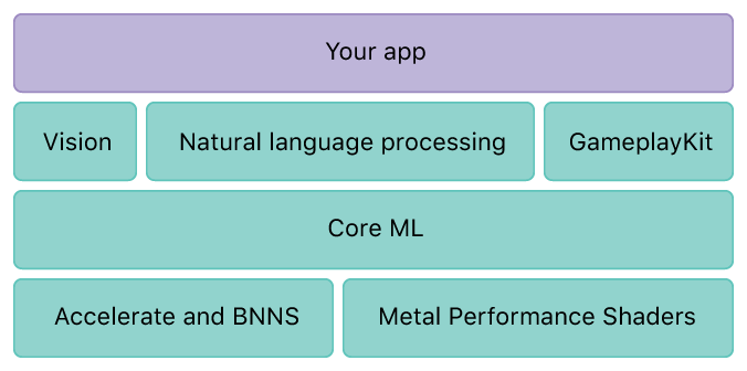
CoreML is able to import a ready-made, trained model (CaffeV1, Keras, scikit-learn) and then provide the developer with the opportunity to export it to the application.
That is, you need to: Build the model on another platform, in Python or C ++, using third-party frameworks. Then train her on a third-party hardware solution.
And only after that you can import and work in Swift language. In my opinion it is very congested and difficult.
Tensorflow
TensorFlow, like other software packages that implement artificial neural networks, has many ready-made abstractions and mechanics for working with neurons, the relationships between them, error calculation and error inverse distribution. But unlike other packages, Jeff Dean (a Google employee, creator of the distributed file system, TensorFlow and many other great solutions) decided to put in TensorFlow the idea of separating the data execution model and the data execution process. This means that first you describe the so-called calculation graph, and only after you start its calculation. This approach allows you to separate and very flexibly work with the data execution model and directly with the data execution process, distributing the execution across different nodes (processors, graphics cards, computers and clusters).
TensorFlowKit
To solve the entire cycle of tasks from model development to working with it in the final application, within the framework of one language, I wrote an access and working interface with TensorFlow.
The architecture of the solution looks like two levels: medium and high.
- At a low C level, the module allows you to access libtensorflow from the swift language.
- The middle level allows you to get away from the C pointers and operate with “beautiful mistakes”.
- A high level implements various abstractions for accessing model elements and various utilities for exporting, importing, and visualizing a graph.
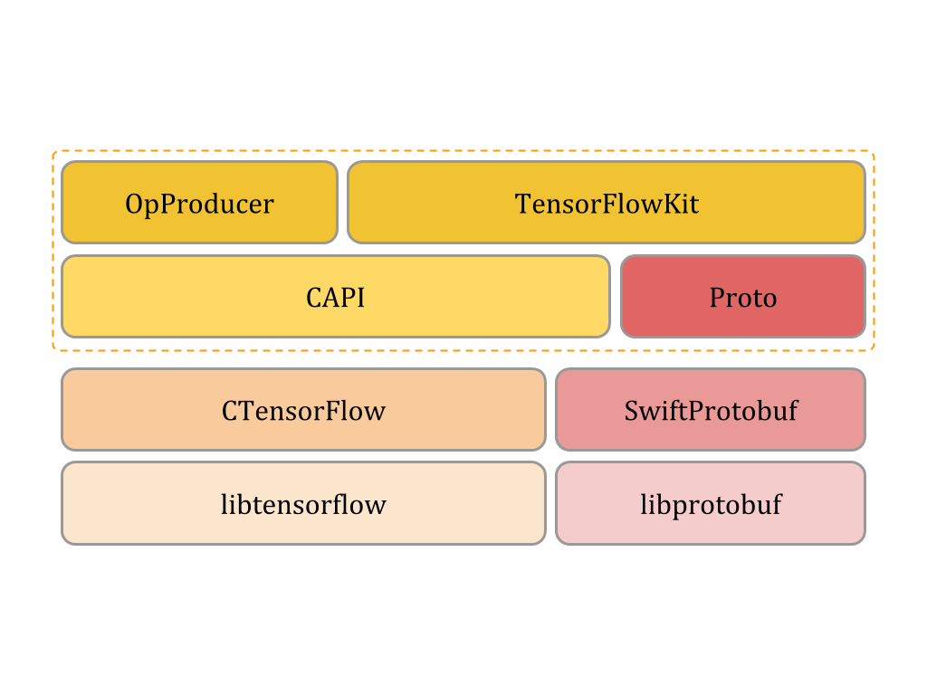
Thus, you can create a model (Graph of calculations) in swift language, train it on a server running Ubuntu OS using several video cards, and then easily open in your program on macOS or tv OS. Development can be carried out in the usual Xcode with all its advantages and disadvantages.
Documentation and API is located at this link.
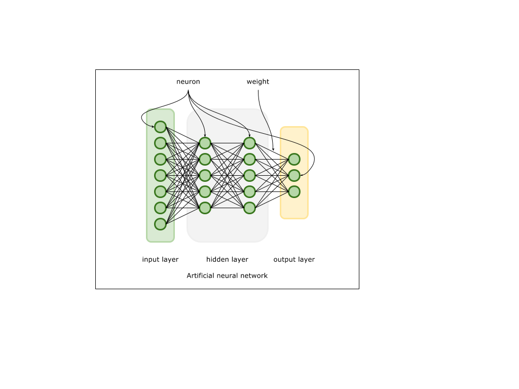
Very briefly about the theory of neural networks.
Artificial neural networks implement a certain (very simplified) model of neuron connections in the tissues of the nervous system. The input signal in the form of a vector of large dimension arrives at the input layer, consisting of neurons. Next, each input neuron transmits this signal to the next layer, transforming it based on the properties of the bonds (weights) between the neurons and the properties of the neurons of the subsequent layers. During training, an output signal is formed on the output layer, which is compared with the expected one. Based on the difference between the output signal and the sample signal, an error value is generated. Further, this error is used to calculate the so-called gradient - a vector in the direction of which it is necessary to correct the connections between neurons so that in the future the neural network produces a signal more similar to what is expected. The process itself is called inverse error distribution or backpropagation. Thus, neurons and the connections between them accumulate the information necessary to generalize the properties of the data model that this neural network is learning. The technical implementation rests on various mathematical operations on matrices and vectors, which in turn have already been implemented to one degree or another by such solutions as BLAS, LAPACK, DSP, etc.
Mnist
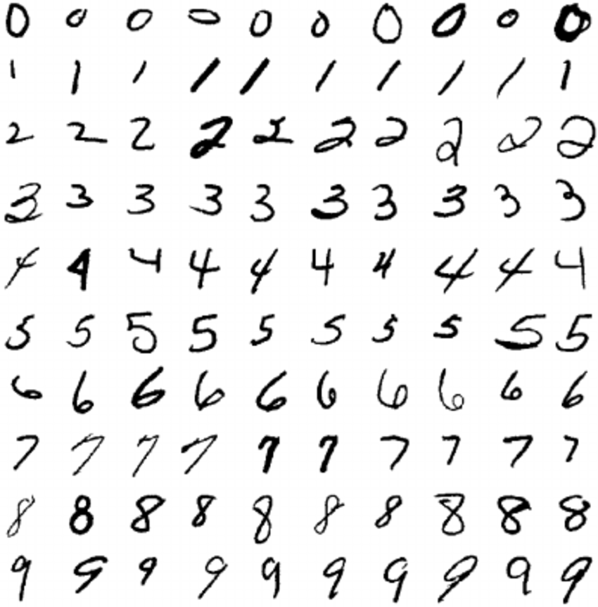
As an example, I took “Hello world!” In the world of neural networks: the problem of classifying images MNIST . The MNIST dataset is thousands of 28 x 28 pixel handwritten image images. Thus, we have ten classes that are neatly distributed in 60,000 images for training and 10,000 images for the test. Our task is to create a neural network capable of classifying an image and determining its belonging to one of ten classes.
Before working with TensorFlowKit itself, you must install TensorFlow. On macOS, you can use the brew package manager:
brew install libtensorflowThe build for linux is available here.
Create a swift project, connect the dependency to it
dependencies: [
    .package(url: "https://github.com/Octadero/TensorFlow.git", from: "0.0.7")
]
We prepare MNIST dataset.
The package for working with the MNIST dataset is written and is available here. The package independently downloads the dataset to a temporary directory, unpacks it and presents it as ready-made classes.
dataset = MNISTDataset(callback: { (error: Error?) in
    print("Ready")
})
We collect the necessary graph of operations.
The entire space and subspace of the computation graph is called Scope and may have its own name.
At the input of our network we will feed two vectors. The first is directly the pictures presented in the form of a vector of higher dimension 784 (28x28 px).
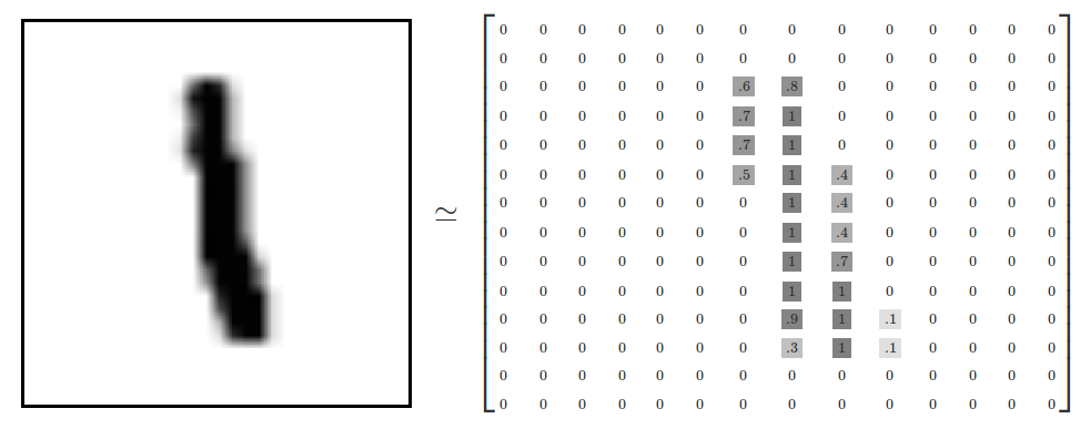
That is, in each component of the vector x there will be a Float value from 0-1, corresponding to the color of the pixel in the picture.
The second vector will be the corresponding class, encrypted in the form (see below) where the corresponding 1 component corresponds to the class number. In this example, the class is 2
[0, 0, 1, 0, 0, 0, 0, 0, 0, 0 ]
Since the input parameters will change during the training process, we create a Placeholder to reference them.
//Input sub scope
let inputScope = scope.subScope(namespace: "input")
let x = try inputScope.placeholder(operationName: "x-input", dtype: Float.self, shape: Shape.dimensions(value: [-1, 784]))
let yLabels = try inputScope.placeholder(operationName: "y-input", dtype: Float.self, shape: Shape.dimensions(value: [-1, 10]))
To visualize the graph, I used TensorBoard . I’ll talk about how to create graphs and visualize the learning process using TensorFlowKit in another article.
On the Input column, it looks like this:
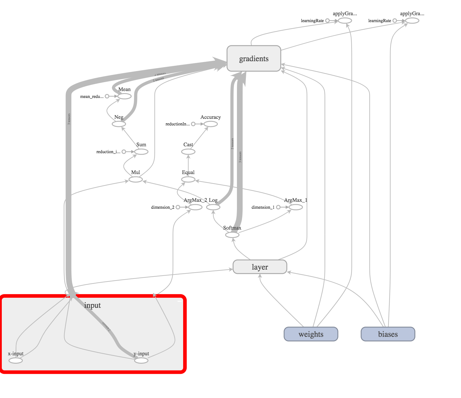
This is our input layer.
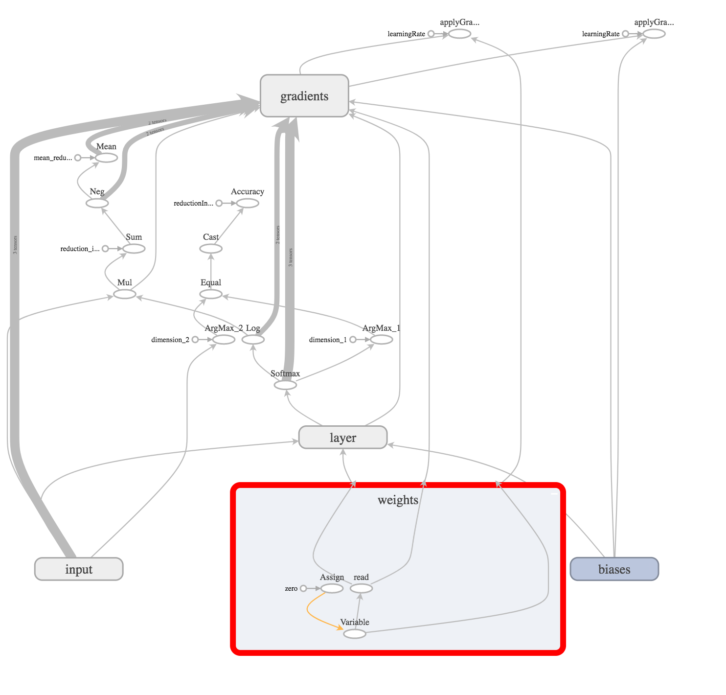
Next, create weights (bonds) between the input layer and the hidden layer.
let weights = try weightVariable(at: scope, name: "weights", shape: Shape.dimensions(value: [784, 10]))
let bias = try biasVariable(at: scope, name: "biases", shape: Shape.dimensions(value: [10]))
Since weights and bases will change (be adjusted) in the process of training the network, we create an operation of variables (variable) in the graph.
And initialize them with a tensor filled with zeros.
Now create a hidden layer that will perform the simplest operation (x * W) + b.
This is the operation of multiplying the vector x (dimension 1x784) by the matrix W (dimension 784x10) and adding a basis.
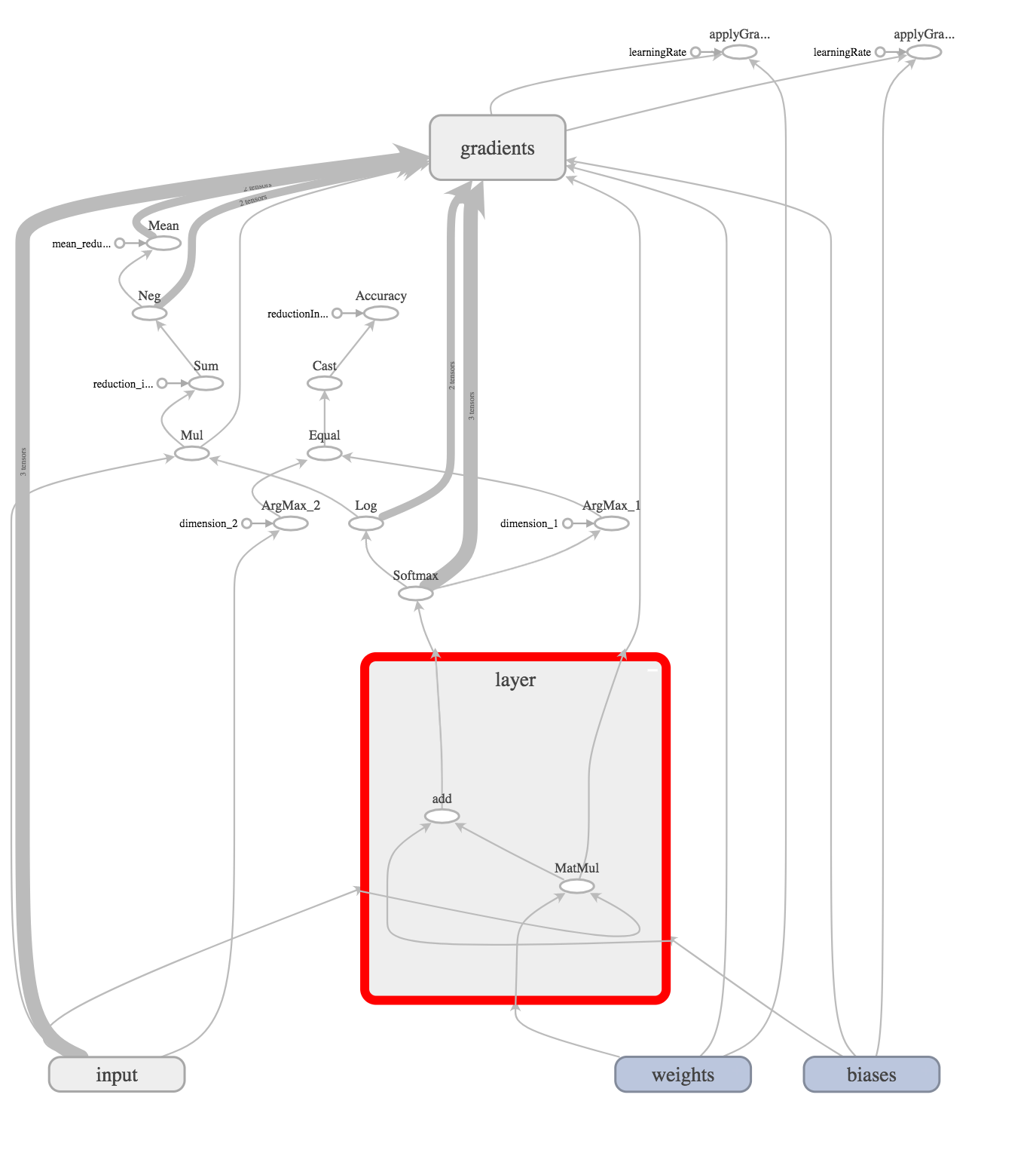
In our case, the hidden layer is already the output (the task of the “Hello World!” Level), so we must analyze the output signal and select the winner. To do this, use the softmax operation.
For a better understanding, what I will describe below, I propose to consider our neural network as a complex function. At the input of our function, the vector x (representing the picture) is received. At the output, we get a vector telling how much the function is sure that the input vector belongs to each of the classes.
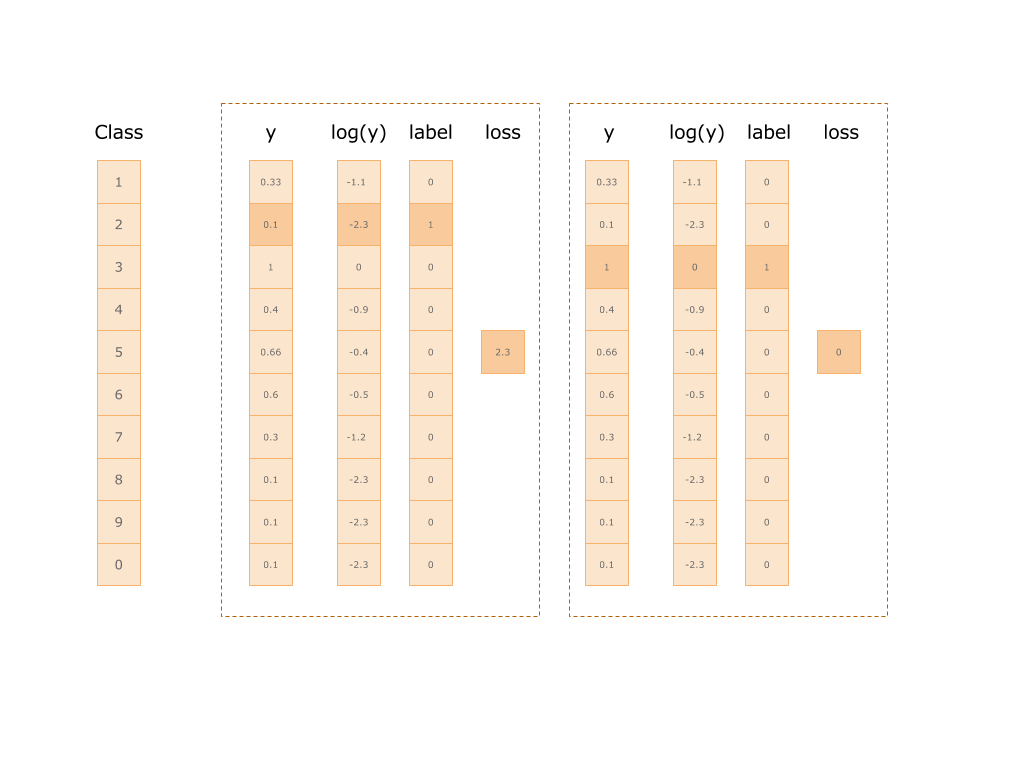
Next, we take the natural logarithm of the magnitude of the predictions obtained in each of the classes and multiply it by the value of the vector of the correct class, neatly transmitted at the very beginning (yLabel).
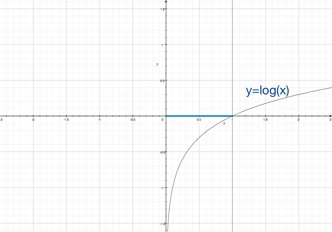
Thus, we get the value of the error and can use it to “condemn” the neural network. Below is a picture of two examples. On the first class 2: the error was 2.3, on the second class 1: the error is zero.
let log = try scope.log(operationName: "Log", x: softmax)
let mul = try scope.mul(operationName: "Mul", x: yLabels, y: log)
let reductionIndices = try scope.addConst(tensor: Tensor(dimensions: [1], values: [Int(1)]), as: "reduction_indices").defaultOutput
let sum = try scope.sum(operationName: "Sum", input: mul, reductionIndices: reductionIndices, keepDims: false, tidx: Int32.self)
let neg = try scope.neg(operationName: "Neg", x: sum)
let meanReductionIndices = try scope.addConst(tensor: Tensor(dimensions: [1], values: [Int(0)]), as: "mean_reduction_indices").defaultOutput
let cross_entropy = try scope.mean(operationName: "Mean", input: neg, reductionIndices: meanReductionIndices, keepDims: false, tidx: Int32.self)
What to do next?
In mathematical terms, we must minimize the objective function. One approach is the gradient descent method. I will try to talk about him in the next article, if necessary.
Thus, we must calculate how much each of the weights (the components of the matrix W) and the basis vector b need to be corrected, so that the neural network makes a smaller error in such input data.
Mathematically, we must find the partial derivatives of the output node by the values of all our intermediate nodes. The resulting symbolic gradients will allow us to “shift” the values of our components of the variables W and b according to how each of them influenced the result of previous calculations.
The magic of TensorFlow.
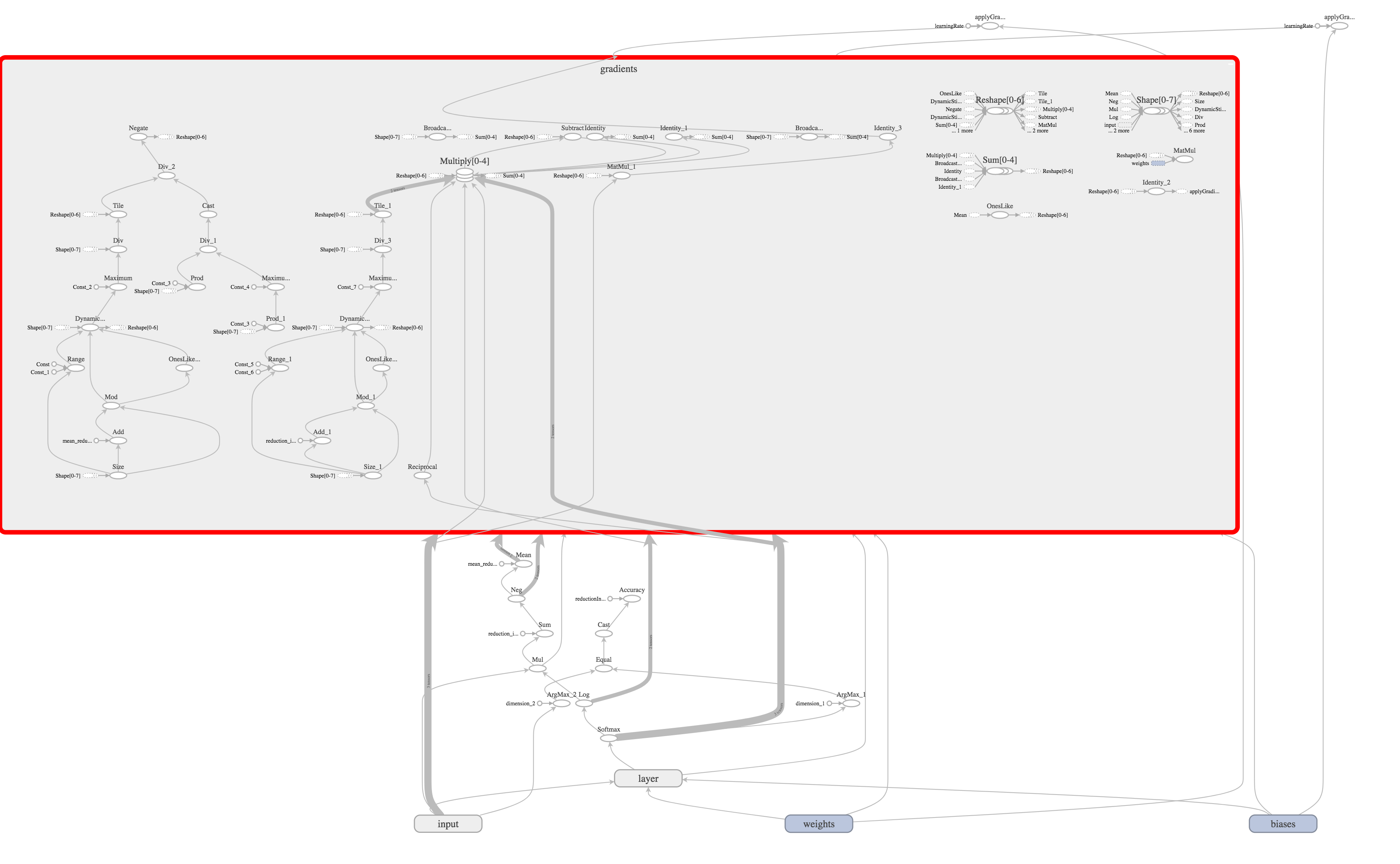
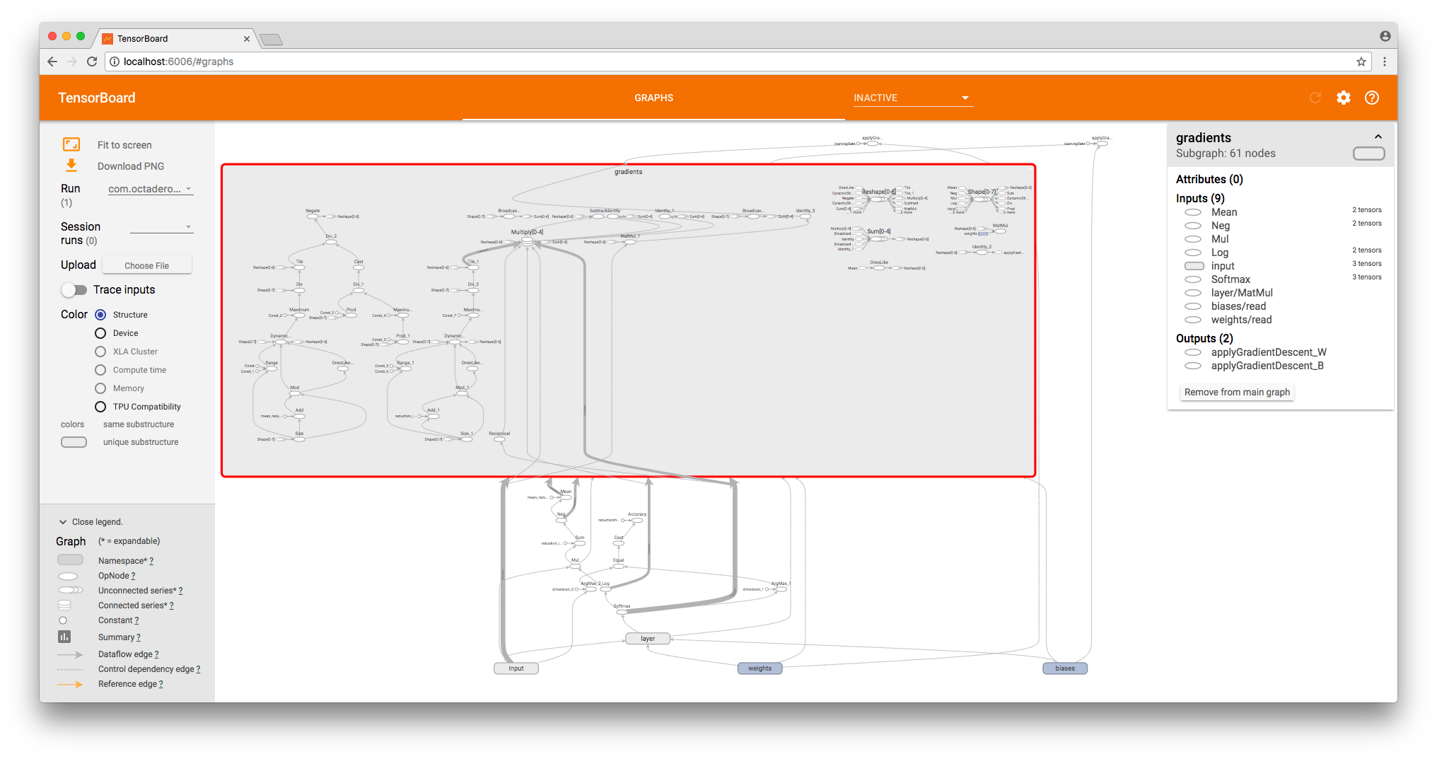
The fact is that everything (in fact, not yet all ) TensorFlow is able to do these complex calculations on its own by analyzing the graph that we built.
let gradientsOutputs = try scope.addGradients(yOutputs: [cross_entropy], xOutputs: [weights.variable, bias.variable])
After calling this operation, TensorFlow will independently build another half hundred operations.
Now it’s enough to add the update operation of our weights to the value calculated earlier by the gradient descent method.
let _ = try scope.applyGradientDescent(operationName: "applyGradientDescent_W",
                                               `var`: weights.variable,
                                               alpha: learningRate,
                                               delta: gradientsOutputs[0],
                                               useLocking: false)
That's it, the count is ready!
As I said, TensorFlow separates model and computation. Therefore, the graph we constructed is only a model for performing calculations.
We can run the calculations using Session.
Having prepared the data from the dataset and placing them in the tensors, we start the session.
guard let dataset = dataset else { throw MNISTTestsError.datasetNotReady }
guard let images = dataset.files(for: .image(stride: .train)).first as? MNISTImagesFile else { throw MNISTTestsError.datasetNotReady }
guard let labels = dataset.files(for: .label(stride: .train)).first as? MNISTLabelsFile else { throw MNISTTestsError.datasetNotReady }
let xTensorInput = try Tensor(dimensions: [bach, 784], values: xs)
let yTensorInput = try Tensor(dimensions: [bach, 10], values: ys)
for index in 0..<1000 {
            let resultOutput = try session.run(inputs: [x, y],
                                               values: [xTensorInput, yTensorInput],
                                               outputs: [loss, applyGradW, applyGradB],
                                               targetOperations: [])
            if index % 100 == 0 {
                let lossTensor = resultOutput[0]
                let gradWTensor = resultOutput[1]
                let gradBTensor = resultOutput[2]
                let wValues: [Float] = try gradWTensor.pullCollection()
                let bValues: [Float] = try gradBTensor.pullCollection()
                let lossValues: [Float] = try lossTensor.pullCollection()
                guard let lossValue = lossValues.first else { continue }
                print("\(index) loss: ", lossValue)
                lossValueResult = lossValue
 print("w max: \(wValues.max()!) min: \(wValues.min()!) b max: \(bValues.max()!) min: \(bValues.min()!)")
            }
        }
This code can be found on GitHub .
Every 100 operations, we deduce, the size of the error.
New article: Visualization of the learning process of a neural network using TensorFlowKit tools has been published.
Only registered users can participate in the survey. Please come in.
What topic would you like to read about next time?
- 10.1% Gradient Descent with TensorFlow 6
- 25.4% Visualization of the graph and the learning process using TensorFlowKit 15
- 27.1% How to make one neural network for Linux, iOS, MacOS, tvOS 16
- 22% More TensorFlowKit 13 Examples
- 15.2% What is the purpose of life 9