BFGS method or one of the most effective optimization methods. Python implementation example

Метод BFGS, итерационный метод численной оптимизации, назван в честь его исследователей: Broyden, Fletcher, Goldfarb, Shanno. Относится к классу так называемых квазиньютоновских методов. В отличие от ньютоновских методов в квазиньютоновских не вычисляется напрямую гессиан функции, т.е. нет необходимости находить частные производные второго порядка. Вместо этого гессиан вычисляется приближенно, исходя из сделанных до этого шагов.

Существует несколько модификаций метода:
L-BFGS (ограниченное использование памяти) — используется в случае большого количества неизвестных.
L-BFGS-B — модификация с ограниченным использованием памяти в многомерном кубе.

The method is effective and stable, therefore it is often used in optimization functions. For example, in SciPy, a popular library for the python language, the optimize function uses BFGS, L-BFGS-B by default.

Algorithm

Let some function be given $$ and we solve the optimization problem: $$.
Where in the general case$$is a non-convex function that has continuous second derivatives.

Step # 1
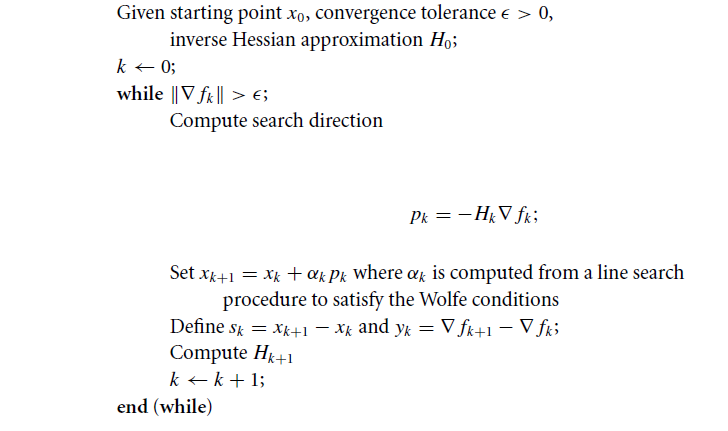
Initialize the starting point$$;
We set the accuracy of the search.$$> 0;
We determine the initial approximation$$where $$- inverse Hessian function;

How to choose the initial approximation$$?
Unfortunately, there is no general formula that works well in all cases. As the initial approximation, we can take the Hessian of the function calculated at the initial point$$. Otherwise, a well-conditioned, non-degenerate matrix can be used; in practice, a single matrix is ​​often taken.

Step No. 2
We find the point in the direction of which we will search, it is determined as follows:

$$

Step №3
Calculate$$ through the recurrence relation:

$$

Coefficient $$ we find using linear search (line search), where $$Satisfies the Wolfe conditions :

$$

$$

Constants $$ and $$ selected as follows: $$. In most implementations:$$ and $$.

In fact, we find this$$ at which the value of the function $$minimally.

Step №4
Determine the vector:

$$

$$

$$ - step of the algorithm in iteration, $$- change the gradient in iteration.

Step # 5
Update the Hessian function, according to the following formula:

$$

Where $$

$$

$$ Is the identity matrix.

Comment

View expression $$is the outer product of two vectors.
Let two vectors be defined$$ and $$then their outer product is equivalent to the matrix product $$. For example, for vectors in the plane:

$$

Step 6
The algorithm continues to be executed until the inequality is true:$$.

Algorithm schematically

Example

Find the extremum of the following function: $$
As a starting point we take $$;
Required accuracy$$;

Find the gradient of the function$$:

$$

Iteration No. 0 :

$$

Find the gradient at the point $$:

$$

Check for the end of the search:

$$

$$

Inequality does not hold, so we continue the iteration process.

We find the point in the direction which we will search:

$$

Where $$Is the identity matrix.

We are looking for this$$$$0 to $$

Analytically, the problem can be reduced to finding the extremum of a function of one variable:

$\$\$\; display\; \$\$\; x\_0\; +\; \alpha \_0\; *\; p\_0\; =\; (1,\; 1)\; +\; \alpha \_0\; (-10,\; 5)\; =\; (1\; -\; 10\alpha \_0,\; 1\; +\; 5\alpha \_0)\; \$\$\; display\; \$\$$

Then

$\$\; inline\; \$\; f\; (\alpha \_0)\; =\; (1\; -\; 10\alpha \_0)\; ^\; 2\; -\; (1\; -\; 10\alpha \_0)\; (1\; +\; 5\alpha \_0)\; +\; (1\; +\; 5\alpha \_0)\; ^\; 2\; +\; 9\; (1\; -\; 10\alpha \_0)\; -\; 6\; (1\; +\; 5\alpha \_0)\; +\; 20\; \$\; inline\; \$$

Simplifying the expression, we find the derivative:

$$

Find the next point $$:

$$

$$

Calculate the value of the gradient in t. $$:

$$

$$

Find the Hessian approximation:

$$

Iteration 1:

$$

$$

Check for the end of the search:

$$

The inequality does not hold, so we continue the iteration process:

$$

$$

We find $$ > 0:

$\$\; inline\; \$\; f\; (\alpha \_1)\; =\; -2.296\alpha \_1\; +\; (-1.913\alpha \_1\; +\; 2.786)\; ^\; 2\; -\; (-1.913\alpha \_1\; +\; 2.786)\; (-\; 1.531\alpha \_1\; -\; 2.571)\; +\; (-1.531\alpha \_1\; -\; 2.571)\; ^\; 2\; -\; 19.86\; \$\; inline\; \$$

$$

Then:

$$

$$

Calculate the value of the gradient at the point $$:

$$

$$

$$

Iteration 2 :

$$

Check for the end of the search:

$$

Inequality is fulfilled hence the search ends. Analytically find the extremum of the function, it is achieved at the point$$.

More about the method

Each iteration can be done with a cost. $$(plus the cost of computing the function and estimating the gradient). There is no$$operations such as solving linear systems or complex mathematical operations. The algorithm is stable and has superlinear convergence, which is sufficient for most practical problems. Even if Newton's methods converge much faster (quadratically), the cost of each iteration is higher, since it is necessary to solve linear systems. The undeniable advantage of the algorithm, of course, is that there is no need to calculate the second derivatives.

Very little theoretically is known about the convergence of the algorithm for the case of a non-convex smooth function, although it is generally accepted that the method works well in practice.

The BFGS formula has self-correcting properties. If the matrix$$incorrectly estimates the curvature of the function and if this poor estimate slows down the algorithm, then the approximation of the Hessian seeks to correct the situation in a few steps. The self-correcting properties of the algorithm work only if the corresponding linear search is implemented (Wolfe conditions are met).

Python implementation example

The algorithm is implemented using the numpy and scipy libraries. A linear search was implemented by using the line_search () function from the scipy.optimize module. In the example, a limit on the number of iterations is imposed.

'''
    Pure Python/Numpy implementation of the BFGS algorithm.
    Reference: https://en.wikipedia.org/wiki/Broyden%E2%80%93Fletcher%E2%80%93Goldfarb%E2%80%93Shanno_algorithm
'''
#!/usr/bin/python
# -*- coding: utf-8 -*-
import numpy as np
import numpy.linalg as ln
import scipy as sp
import scipy.optimize
# Objective function
def f(x):
    return x[0]**2 - x[0]*x[1] + x[1]**2 + 9*x[0] - 6*x[1] + 20
# Derivative
def f1(x):
    return np.array([2 * x[0] - x[1] + 9, -x[0] + 2*x[1] - 6])
def bfgs_method(f, fprime, x0, maxiter=None, epsi=10e-3):
    """
    Minimize a function func using the BFGS algorithm.
    Parameters
    ----------
    func : f(x)
        Function to minimise.
    x0 : ndarray
        Initial guess.
    fprime : fprime(x)
        The gradient of `func`.
    """
    if maxiter is None:
        maxiter = len(x0) * 200
    # initial values
    k = 0
    gfk = fprime(x0)
    N = len(x0)
    # Set the Identity matrix I.
    I = np.eye(N, dtype=int)
    Hk = I
    xk = x0
    while ln.norm(gfk) > epsi and k < maxiter:
        # pk - direction of search
        pk = -np.dot(Hk, gfk)
        # Line search constants for the Wolfe conditions.
        # Repeating the line search
        # line_search returns not only alpha
        # but only this value is interesting for us
        line_search = sp.optimize.line_search(f, f1, xk, pk)
        alpha_k = line_search[0]
        xkp1 = xk + alpha_k * pk
        sk = xkp1 - xk
        xk = xkp1
        gfkp1 = fprime(xkp1)
        yk = gfkp1 - gfk
        gfk = gfkp1
        k += 1
        ro = 1.0 / (np.dot(yk, sk))
        A1 = I - ro * sk[:, np.newaxis] * yk[np.newaxis, :]
        A2 = I - ro * yk[:, np.newaxis] * sk[np.newaxis, :]
        Hk = np.dot(A1, np.dot(Hk, A2)) + (ro * sk[:, np.newaxis] *
                                                 sk[np.newaxis, :])
    return (xk, k)
result, k = bfgs_method(f, f1, np.array([1, 1]))
print('Result of BFGS method:')
print('Final Result (best point): %s' % (result))
print('Iteration Count: %s' % (k))

Thank you for your interest in my article. I hope she was useful to you and you learned a lot.

FUNNYDMAN was with you. Bye everyone!