Meklon July 14, 2017 at 08:38

How we got ahead and calibrated the coffee machine on a spectrophotometer

Once, in the middle of a working day, we suddenly realized that we could no longer live like that. The soul demanded to do something meaningless and merciless in the name of science. And we decided to calibrate the coffee machine. Normal people poke in the default button and drink everything that spills from the coffee maker. A little more advanced for this open the instruction and carefully follow it. Maybe they still read the recommendations of the roaster, unless of course they are rancid noname grains that lay in an unnamed warehouse for a couple of years. We can be classified as normal with a stretch, so we decided to go our own way. In short, under light caffeine intoxication from the seventh cup of espresso, we decided to use the full laboratory arsenal to get a reference drink.

Welcome to the world of madness, ultracentrifuges, spectrophotometry of coffee in special tablets and a small amount of python, pandas and seaborn to visualize all this disgrace.

Proper extraction

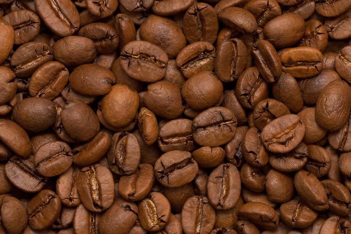
First, we need to understand what we want to get. The main point of proper coffee machine setup is to get a balanced extraction profile. At the same time, not less than half the success depends on the correct grain, which was fried in compliance with all the details of the thermal profile. In horseradish roasters, grains may be unevenly roasted or with other defects. But even perfect coffee can be turned into a terrible swill if it is improperly prepared.

The optimum temperature for the classic way of making coffee is 90-95 ° C. In this case, the number of grains should be approximately 10-20 g / 100 ml of water. It should also be borne in mind that the extraction process is uneven, from lighter and more volatile to less soluble components. The whole trouble is that when we go beyond the optimal values of water temperature, the degree of compression of a coffee tablet (for espresso), the degree of grinding, the ratio of coffee to water or time, we may not have time to “pull out” everything we need from the grain. Or vice versa, capture an excessive amount of heavy fractions, spoiling the taste and balance of the drink. In particular, during hyper-extraction, an excess amount of chlorogenic acids gets into the cup, which cause the coffee to be excessively bitter and shift the taste balance to the acidic side.

Quinic and hydroxycinnamic acids, the structural basis of chlorogenic acids

Experiment preparation

In an automatic coffee machine, only two parameters are available for adjustment: grinding and compression. The degree of grinding is determined by the mechanical rotation of the regulator, which sets the gap between the millstones. Freshly ground coffee tablet compression is pre-installed and has 5 conventional compression levels. Our task is to select the optimal parameters at which the concentration and balance of dissolved substances will give the perfect taste.

The coffee itself for testing was sent to us for inhuman experiments from Torrefacto, for which many thanks to them. Two main categories: B and C (dark and light roast in their classification).

Honduras San Marcos ( source )

Dark roast. We have somehow already switched to medium, but for comparison this variety is a very worthy option. Especially good with milk, but for our tasks we will prepare espresso from it. The taste is quite simple, without subtle nuances, but very rich.

Brazil Ipanema Dulce ( source )

Just a drop dead fragrant variety, with a very balanced taste and sweet fruity sourness. The grain itself contains a large amount of carbohydrates, which gives a light sweetness.

For each variety and each of the five levels of coffee tablet compression, 8 cups of samples are selected. At the same time, laboratory staff spit or rejoice at the result. Blind, naturally. The samples that are optimal in taste are chosen, so that later they can be compared with objective indicators of hardware research.

Deep freeze

We felt sorry for ourselves and we did not drink 80 cups of coffee in one day. Therefore, samples were labeled and thrown into the freezer. Such a cute freezer, with a temperature of about -90 degrees. Eats 4 kilowatts, but in the end, even carbon dioxide falls out in the form of a snowball on the walls. Perfect option.

When all the samples are ready, we take them out of the freezer and put them in an orbital shaker. Yes, I also like the way it sounds. Almost like an orbiting planetary laser, but it's just a shaker. We are waiting for the complete defrosting of the samples and at the same time we mix everything well.

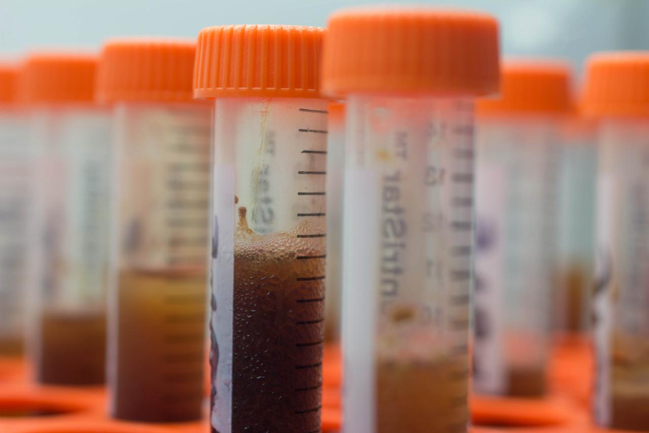
Pour into test tubes and centrifuge

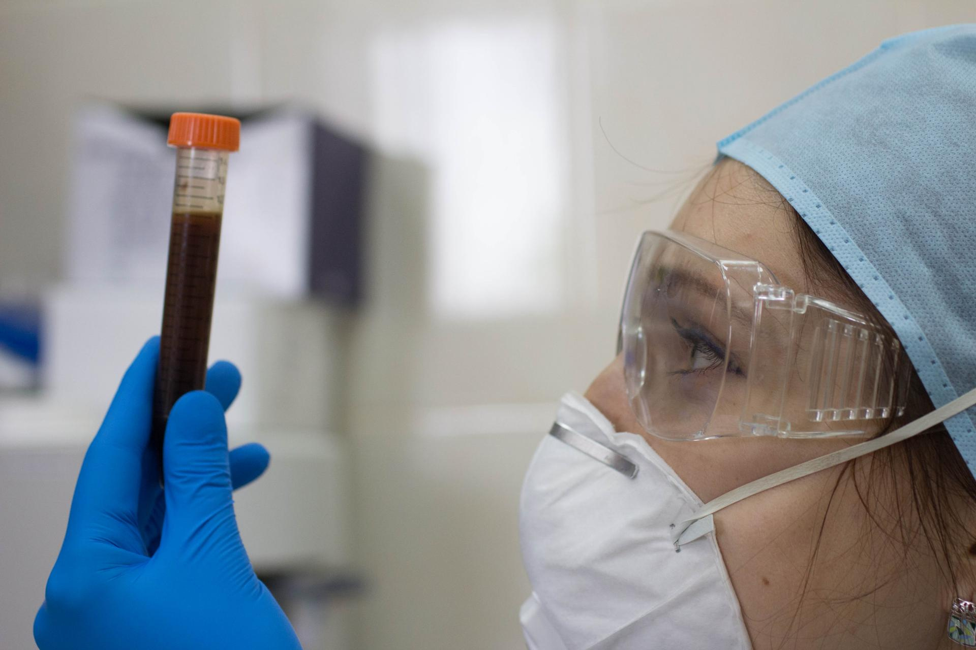
First you need to very carefully examine the samples. Without this miracle, it will not happen)

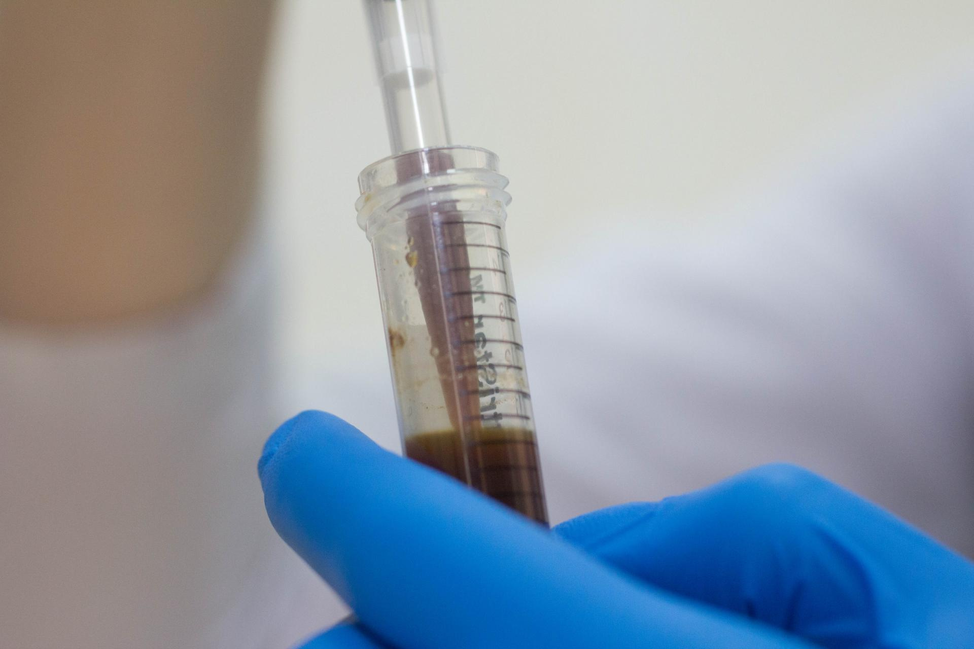
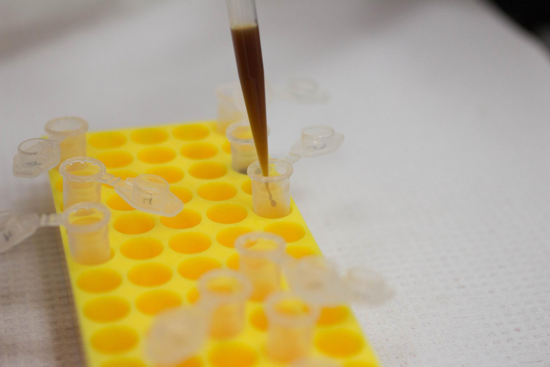
From large test tubes we take coffee with a micropipette and pour into small test tubes for centrifugation. We mark each tube with a number and enter it in a separate journal so as not to mix up the samples later.

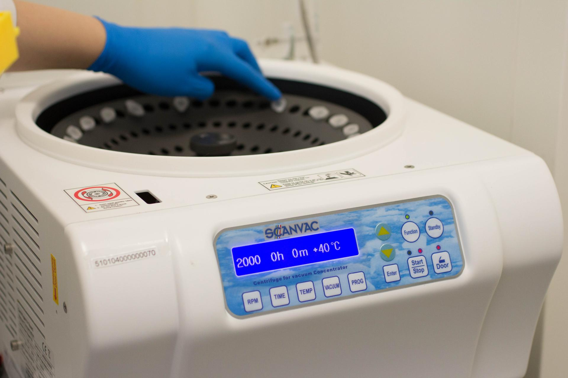
We arrange the tubes in a centrifuge strictly symmetrically to maintain balance. At high speeds, this is critical. After centrifugation, we will get a pure aqueous solution of what was extracted from coffee, and all microparticles that passed through the filter of the coffee machine will remain in the form of sediment.

Spectrophotometry

We again take the micropipette and pour the exact doses of the samples into individual wells of a special 48-well plate.

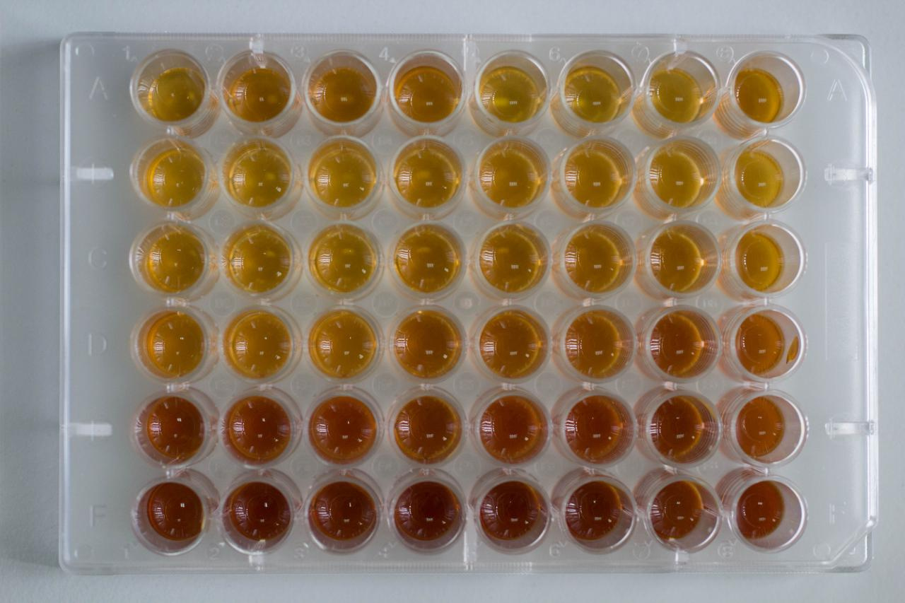
As a result, the samples are beautifully distributed in shades. From top to bottom there is an increase in the degree of compression and the completeness of extraction.

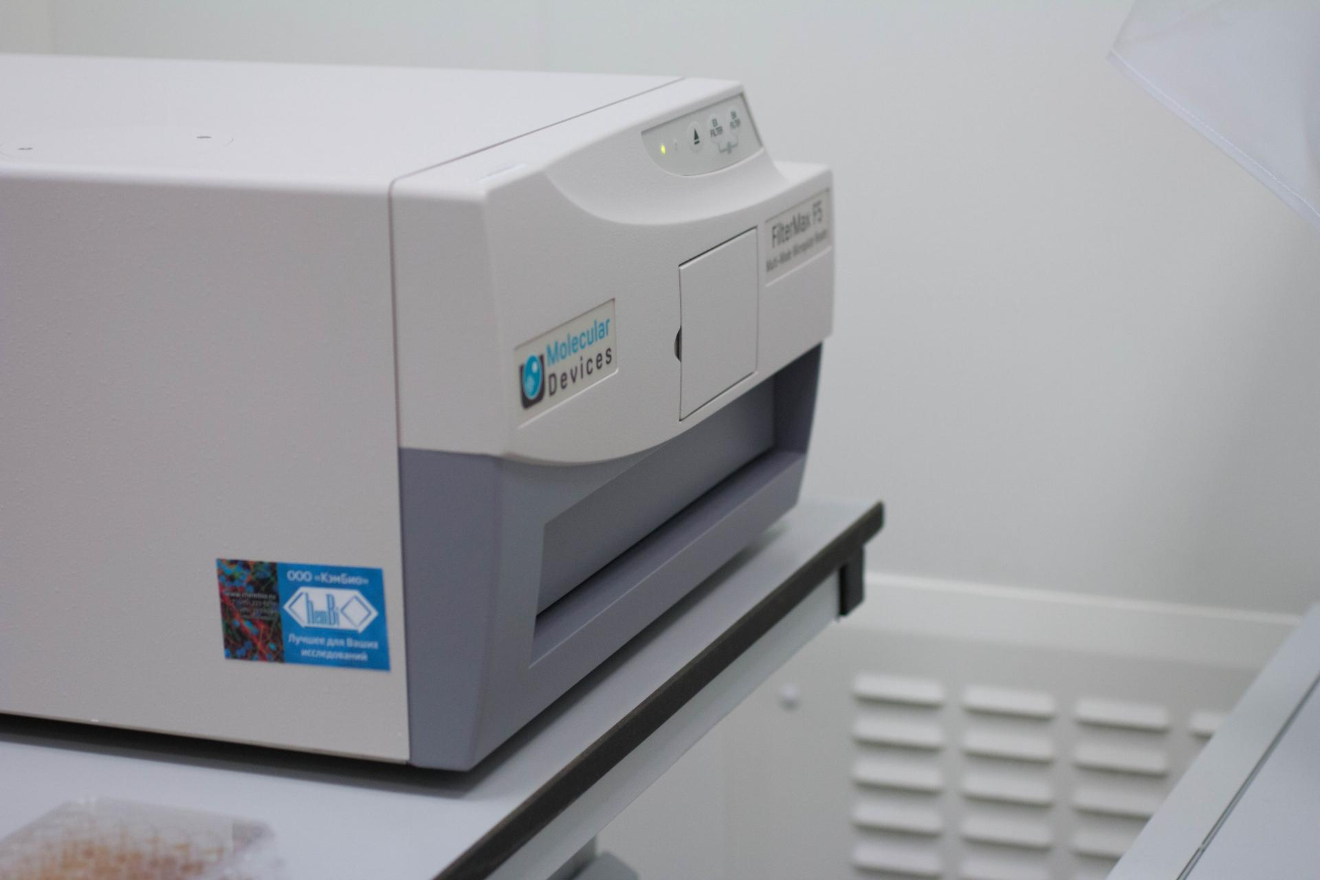
I’m my mom’s operator

The tablets are loaded into a FilterMax spectrophotometer from Molecular Devices. There are a whole bunch of sample research modes, various filter options, laser radiation sources, and the like. We thought for a long time that it would make sense to measure such a strange thing on coffee and decided that measuring the same fluorescence in ultraviolet is rather pointless. We decided to evaluate the degree of absorption of laser radiation at a wavelength of 450 nm. This wavelength is a blue laser. In principle, it is quite logical. A saturated coffee solution has a reddish hue and should absorb the blue part of the spectrum well.

As a result, we obtained absorption tables for all of our samples. However, it would be nice to visualize all of this. Since I most often use python and pandas with seaborn in my work, we will save the data in the most convenient form for loading in pandas.

Percentage absorption in csv format.

Roast, Compression, Absorbance
medium, level 1.21.31
medium, level 1.20.57
medium, level 1.24.49
medium, level 1.26.95
medium, level 1.20.49
medium, level 1.20.06
medium, level 1.21.22
medium, level 1.23.32
medium, level 2.28.09
medium, level 2.28.27
medium, level 2.23.13
medium, level 2.25.72
medium, level 2.26.75
medium, level 2.26.05
medium, level 2.26.92
medium, level 2, 25.92
medium, level 3.32.88
medium, level 3.32.23
medium, level 3.33.13
medium, level 3.28.72
medium, level 3.28.82
medium, level 3.31.49
medium, level 3.32.31
medium, level 3.33.81
medium, level 4,38.68
medium, level 4,40.54
medium, level 4,39.34
medium, level 4,43.3
medium, level 4,41.48
medium, level 4,42.26
medium, level 4,42.73
medium, level 4,42.35
medium, level 5.57.62
medium, level 5.70.62
medium, level 5.70.74
medium, level 5.57.94
medium, level 5.77.62
medium, level 5.76.64
medium, level 5.69.12
medium, level 5.66.39
dark, level 1 , 27.54
dark, level 1.26.8
dark, level 1.30.72
dark, level 1.33.18
dark, level 1.26.72
dark, level 1.26.29
dark, level 1.27.45
dark, level 1.29.55
dark, level 2.34.32
dark, level 2.34.5
dark, level 2.29.36
dark, level 2.31.95
dark, level 2.32.98
dark, level 2.32.28
dark, level 2.33.15
dark, level 2.32.15
dark, level 3.39.11
dark, level 3,38.46
dark, level 3,39.36
dark, level 3,34.95
dark, level 3,35.05
dark, level 3,37.72
dark, level 3,38.54
dark, level 3,40.04
dark, level 4,44.91
dark, level 4 , 46.77
dark, level 4,45.57
dark, level 4,49.53
dark, level 4,47.71
dark, level 4,48.49
dark, level 4,48.96
dark, level 4,48.58
dark, level 5,63.85
dark, level 5,76.85
dark, level 5,76.97
dark, level 5,64.17
dark, level 5,83.85
dark, level 5,82.87
dark, level 5,75.35
dark, level 5,72.62

Draw graphs with python, pandas and seaborn

To plot the chart, we first import our csv as a pandas dataframe. After that, with the help of the wonderful seaborn library and the barplot function, we will build a graph, grouped by degree of frying. For greater contrast, use the "Paired" palette, it is very good when comparing different groups. By the way, as you remember, we ranged the samples according to their taste. The coffee tasters of us are so-so, but surprisingly a consensus has been reached. The optimal taste of the drink was when the degree of absorption at a length of 450 nm was in the region of 32%. We draw the corresponding line on the chart using plt.axhline.

Python code

import matplotlib.pyplot as plt
import pandas as pd
import seaborn as sns
df = pd.read_csv("data.csv")
sns.set()
sns.set_style("whitegrid")
sns.set_context("talk")
ax = sns.barplot(x="Compression", y="Absorbance", hue="Roast", data=df, palette="Paired")
ax.set(ylim=(0, 100), xlabel='Compression level', ylabel='Absorbance at 450 nm, %')
plt.axhline(32, alpha=0.4, color='black', linestyle='dashed', label='Optimal concentration')
plt.legend(loc='upper left')
plt.savefig("plot.png", dpi=300)
plt.show()

The graph clearly shows that the optimal compression ratio for dark roasted coffee is second, and for medium - third. In addition to this amazing conclusion from our experiment, we see that with maximum compression, the dispersion in the concentration of dissolved substances between the individual cups of espresso increases. Either the machine does not provide repeatability, or with such compression, factors such as the length of a randomly punched channel in a coffee tablet through which hot water flows are significantly affected.

To make it finally beautiful, we plot the deviation of our parameter from the optimum. To do this, subtract 32 (our optimum) from the Absorbance column in our dataframe.

# Subtract optimal value
df['Absorbance'] = df['Absorbance'] - 32