Joncker-Volgenant Algorithm + t-SNE = Super-Strength
- Transfer
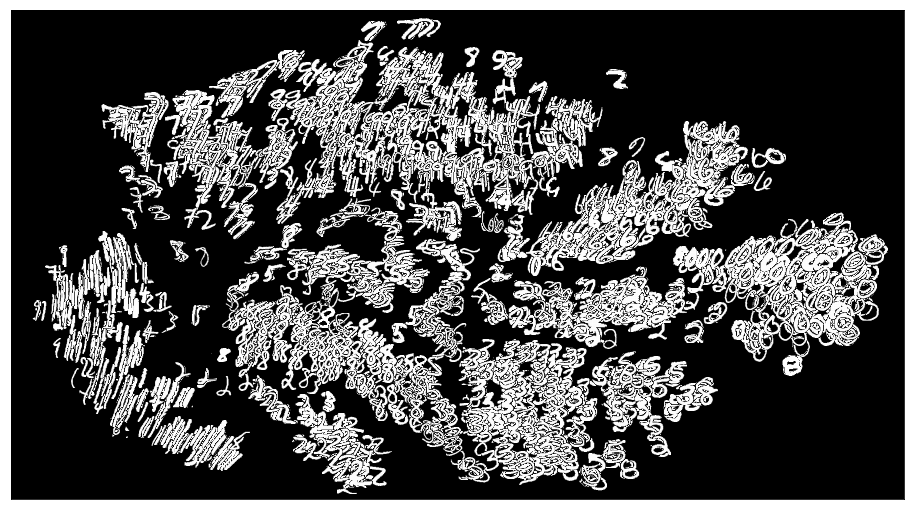
Before:
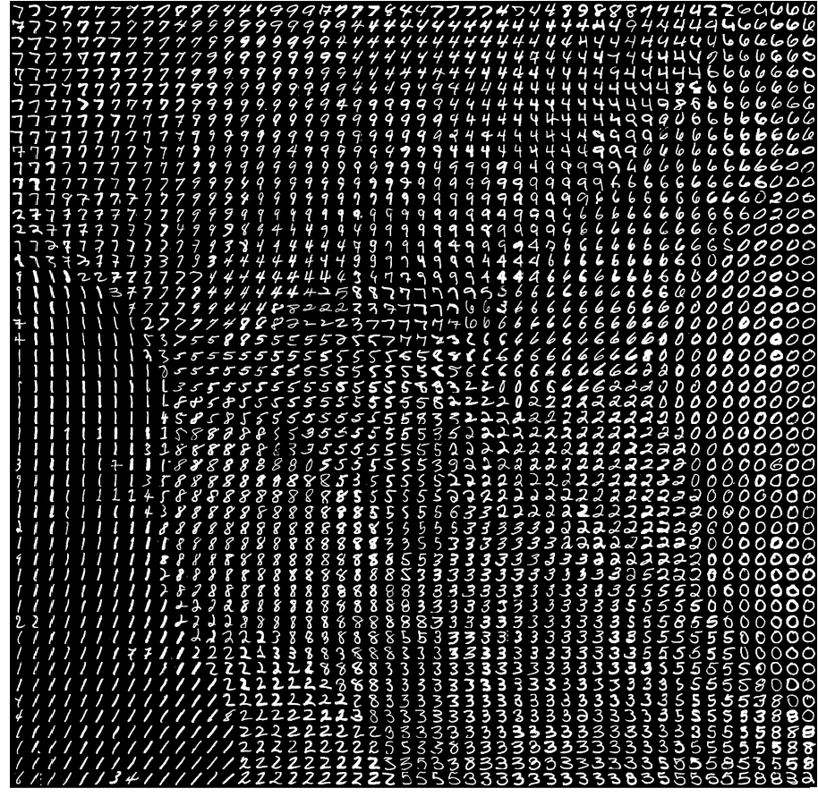
After:
Intrigued? But first things first.
t-SNE is a very popular algorithm that allows you to reduce the dimensionality of your data so that it is easier to visualize. This algorithm can collapse hundreds of measurements to just two, while maintaining important relationships between the data: the closer the objects are located in the original space, the smaller the distance between these objects in the space of reduced dimension. t-SNE works well on small and medium real data sets and does not require a large number of hyperparameter settings. In other words, if we take 100,000 points and pass them through this magical black box, we get a beautiful scatter plot at the output.
Here is a classic example from the field of computer vision. There is a well-known dataset called MNISTcreated by Jan Lekun (one of the creators of the algorithm for training neural networks by the method of back propagation of error - the basis of modern deep learning) and others. It is often used as a universal data set for evaluating ideas related to neural networks, as well as in scientific research. MNIST is 70,000 28x28 black and white images. Each of them is a scan of a handwritten digit from the segment [0, 9]. There is a way to get an “ infinite ” set of MNIST, but I will not deviate from the topic.
Thus, the MNIST sample contains sign and can be represented as a 784-dimensional vector. The vectors are linear, and in this interpretation we lose the relationship of location between the individual pixels, but still it is useful. If you try to imagine what our data set looks like in 784D, you can go crazy if you are not a specially trained mathematician. Ordinary people can only consume information in 3D, 2D, or 1D dimensions. Implicitly, you can add another dimension - time, but it is unlikely that someone will say that the computer display is 3D only because it updates the picture with a frequency of 100 Hz. Therefore, it would be great to know a way to display 784 measurements in two. Sounds impossible? In general, it is. The Dirichlet principle comes into play : what kind of mapping we will not choose, collisions cannot be avoided.

3D Illusion -> 2D Projection in Shadowmatic
Fortunately, the following suggestions can be made:
The question arises: what is the best approximating problem in paragraph 2? Unfortunately, there is no “best”. The quality of dimensionality reduction is subjective and depends on your final goal, as well as when choosing a clustering method.
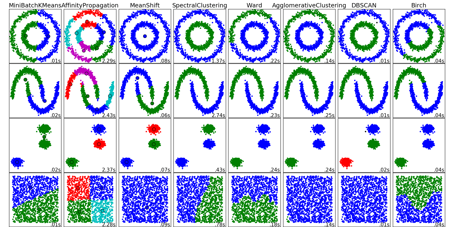
Different clustering algorithms from sklearn
t-SNE are one of the possible dimensionality reduction algorithms, which are called embedded graph algorithms. The key idea is to maintain a “similarity” relationship. Try it yourself .
These are all artificial examples, they are good, but not enough. Most real data sets resemble a cloud with conical clusters. For example, MNIST looks like this.
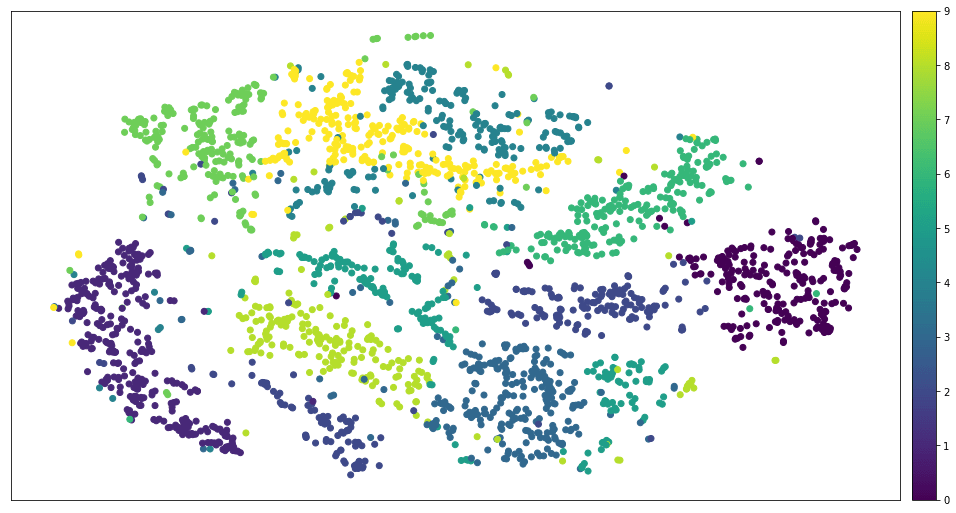
MNIST after applying t-SNE
Now let's sharply turn aside and get acquainted with the concept of linear programming (LP). Sorry, this is not a new design pattern, Javascript framework or startup. This is the math:
We minimize the scalar product and
and  taking into account the system of linear inequalities depending on , and the requirements that all its coordinates are non-negative. LP is a well-studied topic in the theory of convex optimization; as you know, this problem is solved in a weakly polynomial time - usually in
 where n is the number of variables (task dimension). But there are approximating algorithms that run in linear time. These algorithms use matrix multiplication and can be effectively parallelized. Paradise for the programmer!
Surprisingly many tasks can be reduced to LP. Take, for example, the transportation problem .

Transport task: points of departure (S) and points of consumption (D)
There are a number of points of departure and points of consumption that may be unequal. Each point of consumption needs a certain quantity of goods. Each point of departure has limited resources and is associated with some points of consumption. The main task is as follows: each edge has its value
  Therefore, it is necessary to find the distribution of supplies with minimal costs.
Strictly speaking,
The last condition means that either at the points of departure the goods will end, or the demand for goods will run out. If , expression 8 can be normalized and simplified as follows:
If we replace “shipment” and “consumption” with “land”, then will lead us to the task of the mover ( Earth Mover's Distance , EMD): to minimize the work required to drag the earth from one set of heaps to another. Now you know what to do if you have to dig holes in the ground.
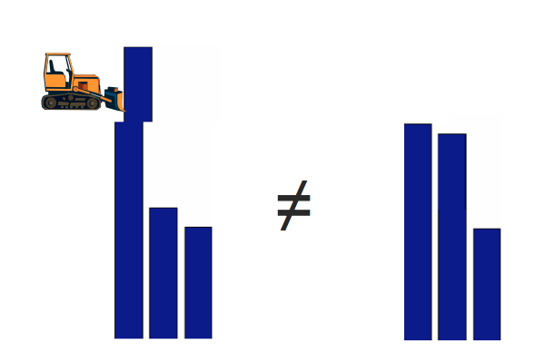
Earth Mover's Distance
If we replace “departure” and “consumption” with “histograms”, we get the most common way to compare images from the “before deep learning” era ( example article ). This method is better than naive L2, since it takes into account not only differences in absolute value, but also a difference in location.

EMD is better at comparing histograms than Euclidean distance
If we replace “departure” and “consumption” with the words that we will come to Word Mover's Distance, an effective way to compare the meanings of two sentences using word2vec to get vector representations of words.

Word Mover's Distance.
If we relax conditions 5-8 , throwing 8 , taking and turning inequality 6 and 7 into equation adding them symmetrical inequality, we obtain a task assignment (Linear Assignment Problem, LAP):
In contrast to the transportation problem, we can prove that - The solution is always binary. In other words, either all goods from points of departure go to points of consumption, or nothing goes anywhere.
As we understood from the first section, t-SNE, like all laying algorithms on a plane, produces a scattering diagram at the output. Although this is ideal for the task of researching data sets, sometimes there is a need to lay the original diagram on the correct grid. For example, such styling is necessary source {d} ... we will soon find out why.

The correct grid
After applying t-SNE, instead of the dots we will draw the numbers MNIST; here's what it looks like:
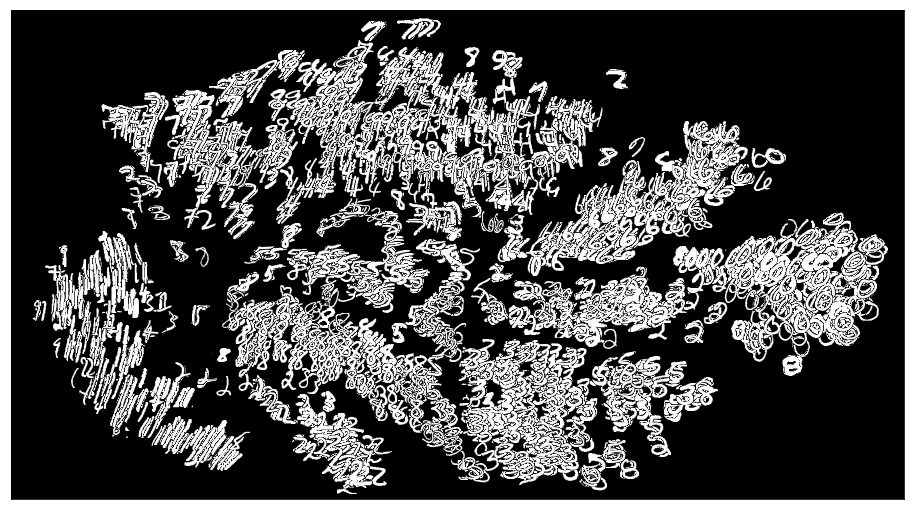
MNIST digits after t-SNE
Not too clear. This is where LAP arises: you can define a cost matrix as a pair Euclidean distance between t-SNE samples and grid nodes, set the grid area equal to the size of the data set , and as a result, we solve the problem. But how? We have not yet talked about any algorithm.
It turns out that there are a huge number of general-purpose linear optimization algorithms, starting with the simplex method and ending with extremely complex tools. Algorithms developed specifically for a specific task usually converge much faster, although they have some limitations.
The Hungarian algorithm is one of the specialized methods developed in the 1950s. Its complexity is. It is quite simple to understand and implement, and therefore popular in many projects. For example, he recently became part of sсipy . Unfortunately, it does not work fast on large amounts of data, and the scipy option is especially slow. I waited an hour to process 2500 MNIST samples, and Python was still digesting the victim.
Algorithm-Volgenanta Jonker ( Jonker-Volgenant , JV) - improved approach developed in 1987. It is based on a shortest path also passing augmentalnoy chain, and its complexity is also cubic, but it using some of tricks, dramatically reduces the computational load. The performance of many graph-laying algorithms, including JV, was extensively examined in a 2000 article by Discrete Applied Mathematics. The conclusion was as follows:
However, JV also has a drawback. He is very tolerant of differences between pairs of elements in the cost matrix. For example, if we look for the shortest path in a graph using the Dijkstra algorithm, and two very similar costs appear on this graph, the algorithm runs the risk of going into an infinite loop. If we take a close look at Dijkstra’s algorithm, we’ll find that when the accuracy limit of floating point values is reached, terrible things can happen. The usual way out of the situation is to multiply the cost matrix by some large number.
Still, the most tempting thing in JV for such a lazy engineer like me is the Python 2 package, which is a wrapper of an ancient implementation of the algorithm in C: pyLAPJV . This C code was written by Roy Jonkerin 1996 for the company MagicLogic Optimization, of which he is president. In addition to the fact that pyLAPJV is no longer supported, it has a minor data output problem that I fixed in pull request # 2 . C code is reliable, but it does not use multithreading or SIMD instructions. Of course, we understand that the JV is single-threaded by nature, and it is not so easy to parallelize it, however, I managed to speed it up almost twice, optimizing the most expensive stage - cutting the augmentation chain - using AVX2 . The result is the src-d / lapjv package in Python 3, available under the MIT license.
The reduction of the augmented chain basically boils down to finding the minimum and second minimum elements in the array. It sounds simple, as it actually is, unoptimized C code takes 20 lines. The AVX version is 4 times larger: we send minimum values to each SIMD processor element, perform blending , and then apply some other SIMD black magic spells that I learned while working on Samsung's libSoundFeatureExtraction .
Finding two consecutive minimum values, C ++
Finding two consecutive minimum values, optimized code with instructions AVX2
On my laptop lapjv stacks 2500 MNIST samples in 5 seconds, and here it is a precious result:
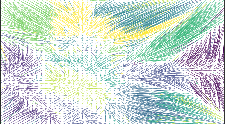
Solving the assignment problem for MNIST after t-SNE
To prepare this post, I used the Jupiter Notebook (source here ).
There is an effective way to lay t-SNE-treated samples on the correct grid. It is based on solving the assignment problem (LAP) using the Jonker-Volgenant algorithm implemented in src-d / lapjv . This algorithm can be scaled to 10,000 samples.
After:
Intrigued? But first things first.
t-SNE
t-SNE is a very popular algorithm that allows you to reduce the dimensionality of your data so that it is easier to visualize. This algorithm can collapse hundreds of measurements to just two, while maintaining important relationships between the data: the closer the objects are located in the original space, the smaller the distance between these objects in the space of reduced dimension. t-SNE works well on small and medium real data sets and does not require a large number of hyperparameter settings. In other words, if we take 100,000 points and pass them through this magical black box, we get a beautiful scatter plot at the output.
Here is a classic example from the field of computer vision. There is a well-known dataset called MNISTcreated by Jan Lekun (one of the creators of the algorithm for training neural networks by the method of back propagation of error - the basis of modern deep learning) and others. It is often used as a universal data set for evaluating ideas related to neural networks, as well as in scientific research. MNIST is 70,000 28x28 black and white images. Each of them is a scan of a handwritten digit from the segment [0, 9]. There is a way to get an “ infinite ” set of MNIST, but I will not deviate from the topic.
Thus, the MNIST sample contains
sign and can be represented as a 784-dimensional vector. The vectors are linear, and in this interpretation we lose the relationship of location between the individual pixels, but still it is useful. If you try to imagine what our data set looks like in 784D, you can go crazy if you are not a specially trained mathematician. Ordinary people can only consume information in 3D, 2D, or 1D dimensions. Implicitly, you can add another dimension - time, but it is unlikely that someone will say that the computer display is 3D only because it updates the picture with a frequency of 100 Hz. Therefore, it would be great to know a way to display 784 measurements in two. Sounds impossible? In general, it is. The Dirichlet principle comes into play : what kind of mapping we will not choose, collisions cannot be avoided.3D Illusion -> 2D Projection in Shadowmatic
Fortunately, the following suggestions can be made:
- The initial multidimensional space is sparse , that is, it is unlikely to be uniformly filled with samples.
- We do not need to find the exact mapping, especially knowing that it does not exist. Instead, you can solve another problem that has a guaranteed exact solution and approximates the expected result. This is reminiscent of the principle of JPEG compression: the result is never exactly identical, but the image looks very similar to the original.
The question arises: what is the best approximating problem in paragraph 2? Unfortunately, there is no “best”. The quality of dimensionality reduction is subjective and depends on your final goal, as well as when choosing a clustering method.
Different clustering algorithms from sklearn
t-SNE are one of the possible dimensionality reduction algorithms, which are called embedded graph algorithms. The key idea is to maintain a “similarity” relationship. Try it yourself .
These are all artificial examples, they are good, but not enough. Most real data sets resemble a cloud with conical clusters. For example, MNIST looks like this.
MNIST after applying t-SNE
Line programming
Now let's sharply turn aside and get acquainted with the concept of linear programming (LP). Sorry, this is not a new design pattern, Javascript framework or startup. This is the math:


We minimize the scalar product
and taking into account the system of linear inequalities depending on , and the requirements that all its coordinates are non-negative. LP is a well-studied topic in the theory of convex optimization; as you know, this problem is solved in a weakly polynomial time - usually inwhere n is the number of variables (task dimension). But there are approximating algorithms that run in linear time. These algorithms use matrix multiplication and can be effectively parallelized. Paradise for the programmer! Surprisingly many tasks can be reduced to LP. Take, for example, the transportation problem .
Transport task: points of departure (S) and points of consumption (D)
There are a number of points of departure and points of consumption that may be unequal. Each point of consumption needs a certain quantity of goods. Each point of departure has limited resources and is associated with some points of consumption. The main task is as follows: each edge
has its value Therefore, it is necessary to find the distribution of supplies with minimal costs. Strictly speaking,


The last condition means that either at the points of departure the goods will end, or the demand for goods will run out. If
, expression 8 can be normalized and simplified as follows:
If we replace “shipment” and “consumption” with “land”, then
will lead us to the task of the mover ( Earth Mover's Distance , EMD): to minimize the work required to drag the earth from one set of heaps to another. Now you know what to do if you have to dig holes in the ground. Earth Mover's Distance
If we replace “departure” and “consumption” with “histograms”, we get the most common way to compare images from the “before deep learning” era ( example article ). This method is better than naive L2, since it takes into account not only differences in absolute value, but also a difference in location.
EMD is better at comparing histograms than Euclidean distance
If we replace “departure” and “consumption” with the words that we will come to Word Mover's Distance, an effective way to compare the meanings of two sentences using word2vec to get vector representations of words.
Word Mover's Distance.
If we relax conditions 5-8 , throwing 8 , taking
and turning inequality 6 and 7 into equation adding them symmetrical inequality, we obtain a task assignment (Linear Assignment Problem, LAP):


In contrast to the transportation problem, we can prove that
- The solution is always binary. In other words, either all goods from points of departure go to points of consumption, or nothing goes anywhere.t-SNE LAP
As we understood from the first section, t-SNE, like all laying algorithms on a plane, produces a scattering diagram at the output. Although this is ideal for the task of researching data sets, sometimes there is a need to lay the original diagram on the correct grid. For example, such styling is necessary source {d} ... we will soon find out why.
The correct grid
After applying t-SNE, instead of the dots we will draw the numbers MNIST; here's what it looks like:
MNIST digits after t-SNE
Not too clear. This is where LAP arises: you can define a cost matrix as a pair Euclidean distance between t-SNE samples and grid nodes, set the grid area equal to the size of the data set
, and as a result, we solve the problem. But how? We have not yet talked about any algorithm.Joncker-Volgenant Algorithm
It turns out that there are a huge number of general-purpose linear optimization algorithms, starting with the simplex method and ending with extremely complex tools. Algorithms developed specifically for a specific task usually converge much faster, although they have some limitations.
The Hungarian algorithm is one of the specialized methods developed in the 1950s. Its complexity is
. It is quite simple to understand and implement, and therefore popular in many projects. For example, he recently became part of sсipy . Unfortunately, it does not work fast on large amounts of data, and the scipy option is especially slow. I waited an hour to process 2500 MNIST samples, and Python was still digesting the victim. Algorithm-Volgenanta Jonker ( Jonker-Volgenant , JV) - improved approach developed in 1987. It is based on a shortest path also passing augmentalnoy chain, and its complexity is also cubic, but it using some of tricks, dramatically reduces the computational load. The performance of many graph-laying algorithms, including JV, was extensively examined in a 2000 article by Discrete Applied Mathematics. The conclusion was as follows:
“JV has a good and stable average performance for all classes (tasks - author's note), and this is the best algorithm for both random and specific tasks.”
However, JV also has a drawback. He is very tolerant of differences between pairs of elements in the cost matrix. For example, if we look for the shortest path in a graph using the Dijkstra algorithm, and two very similar costs appear on this graph, the algorithm runs the risk of going into an infinite loop. If we take a close look at Dijkstra’s algorithm, we’ll find that when the accuracy limit of floating point values is reached, terrible things can happen. The usual way out of the situation is to multiply the cost matrix by some large number.
Still, the most tempting thing in JV for such a lazy engineer like me is the Python 2 package, which is a wrapper of an ancient implementation of the algorithm in C: pyLAPJV . This C code was written by Roy Jonkerin 1996 for the company MagicLogic Optimization, of which he is president. In addition to the fact that pyLAPJV is no longer supported, it has a minor data output problem that I fixed in pull request # 2 . C code is reliable, but it does not use multithreading or SIMD instructions. Of course, we understand that the JV is single-threaded by nature, and it is not so easy to parallelize it, however, I managed to speed it up almost twice, optimizing the most expensive stage - cutting the augmentation chain - using AVX2 . The result is the src-d / lapjv package in Python 3, available under the MIT license.
The reduction of the augmented chain basically boils down to finding the minimum and second minimum elements in the array. It sounds simple, as it actually is, unoptimized C code takes 20 lines. The AVX version is 4 times larger: we send minimum values to each SIMD processor element, perform blending , and then apply some other SIMD black magic spells that I learned while working on Samsung's libSoundFeatureExtraction .
template
__attribute__((always_inline)) inline
std::tuple find_umins(
    idx dim, idx i, const cost *assigncost, const cost *v) {
  cost umin = assigncost[i * dim] - v[0];
  idx j1 = 0;
  idx j2 = -1;
  cost usubmin = std::numeric_limits::max();
  for (idx j = 1; j < dim; j++) {
    cost h = assigncost[i * dim + j] - v[j];
    if (h < usubmin) {
      if (h >= umin) {
        usubmin = h;
        j2 = j;
      } else {
        usubmin = umin;
        umin = h;
        j2 = j1;
        j1 = j;
      }
    }
  }
  return std::make_tuple(umin, usubmin, j1, j2);
}
Finding two consecutive minimum values, C ++
Show code
template
__attribute__((always_inline)) inline
std::tuple find_umins(
    idx dim, idx i, const float *assigncost, const float *v) {
  __m256i idxvec = _mm256_setr_epi32(0, 1, 2, 3, 4, 5, 6, 7);
  __m256i j1vec = _mm256_set1_epi32(-1), j2vec = _mm256_set1_epi32(-1);
  __m256 uminvec = _mm256_set1_ps(std::numeric_limits::max()),
         usubminvec = _mm256_set1_ps(std::numeric_limits::max());
  for (idx j = 0; j < dim - 7; j += 8) {
    __m256 acvec = _mm256_loadu_ps(assigncost + i * dim + j);
    __m256 vvec = _mm256_loadu_ps(v + j);
    __m256 h = _mm256_sub_ps(acvec, vvec);
    __m256 cmp = _mm256_cmp_ps(h, uminvec, _CMP_LE_OQ);
    usubminvec = _mm256_blendv_ps(usubminvec, uminvec, cmp);
    j2vec = _mm256_blendv_epi8(
        j2vec, j1vec, reinterpret_cast<__m256i>(cmp));
    uminvec = _mm256_blendv_ps(uminvec, h, cmp);
    j1vec = _mm256_blendv_epi8(
        j1vec, idxvec, reinterpret_cast<__m256i>(cmp));
    cmp = _mm256_andnot_ps(cmp, _mm256_cmp_ps(h, usubminvec, _CMP_LT_OQ));
    usubminvec = _mm256_blendv_ps(usubminvec, h, cmp);
    j2vec = _mm256_blendv_epi8(
        j2vec, idxvec, reinterpret_cast<__m256i>(cmp));
    idxvec = _mm256_add_epi32(idxvec, _mm256_set1_epi32(8));
  }
  float uminmem[8], usubminmem[8];
  int32_t j1mem[8], j2mem[8];
  _mm256_storeu_ps(uminmem, uminvec);
  _mm256_storeu_ps(usubminmem, usubminvec);
  _mm256_storeu_si256(reinterpret_cast<__m256i*>(j1mem), j1vec);
  _mm256_storeu_si256(reinterpret_cast<__m256i*>(j2mem), j2vec);
  idx j1 = -1, j2 = -1;
  float umin = std::numeric_limits::max(),
        usubmin = std::numeric_limits::max();
  for (int vi = 0; vi < 8; vi++) {
    float h = uminmem[vi];
    if (h < usubmin) {
      idx jnew = j1mem[vi];
      if (h >= umin) {
        usubmin = h;
        j2 = jnew;
      } else {
        usubmin = umin;
        umin = h;
        j2 = j1;
        j1 = jnew;
      }
    }
  }
  for (int vi = 0; vi < 8; vi++) {
    float h = usubminmem[vi];
    if (h < usubmin) {
      usubmin = h;
      j2 = j2mem[vi];
    }
  }
  for (idx j = dim & 0xFFFFFFF8u; j < dim; j++) {
    float h = assigncost[i * dim + j] - v[j];
    if (h < usubmin) {
      if (h >= umin) {
        usubmin = h;
        j2 = j;
      } else {
        usubmin = umin;
        umin = h;
        j2 = j1;
        j1 = j;
      }
    }
  }
  return std::make_tuple(umin, usubmin, j1, j2);
}
Finding two consecutive minimum values, optimized code with instructions AVX2
On my laptop lapjv stacks 2500 MNIST samples in 5 seconds, and here it is a precious result:
Solving the assignment problem for MNIST after t-SNE
Notebook
To prepare this post, I used the Jupiter Notebook (source here ).
Conclusion
There is an effective way to lay t-SNE-treated samples on the correct grid. It is based on solving the assignment problem (LAP) using the Jonker-Volgenant algorithm implemented in src-d / lapjv . This algorithm can be scaled to 10,000 samples.
Oh, and come to us to work? :)wunderfund.io is a young foundation that deals with high-frequency algorithmic trading . High-frequency trading is a continuous competition of the best programmers and mathematicians around the world. By joining us, you will become part of this fascinating battle.
We offer interesting and complex data analysis and low latency development tasks for enthusiastic researchers and programmers. A flexible schedule and no bureaucracy, decisions are quickly taken and implemented.
Join our team: wunderfund.io