Automated python code visualization. Part two: implementation
The first part of the article briefly discussed the flowcharts and the available tools for working with them. Then all the graphic primitives needed to create a graphical representation of the code were discussed. An example of an environment that supports this graphical representation is shown in the image below.
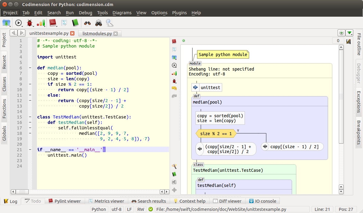
Environment that supports graphical representation of code
In the second part, we will focus on the implementation, performed mainly on Python. Implemented and planned functionality, as well as the proposed micro markup language, will be discussed.
The technology was implemented as part of an open source project called Codimension . All source code is available under the GPL v.3 license and is hosted in three repositories on github : two Python extension modules cdm-pythonparser and cdm-flowparser plus the IDE itself . The extension modules are mainly written in C / C ++, and the IDE in Python series 2. For the graphic part, the Python wrapper of the QT library - PyQT was used.
Development is done on Linux and for Linux. The main distribution used was Ubuntu.
The environment is designed to work with projects written in Python series 2.
The diagram below shows the IDE architecture.
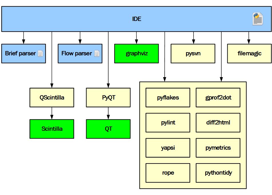
Architecture IDE
Blue on the diagram indicates the parts developed in the project. Yellow - third-party Python modules, and green - third-party binary modules.
From the very beginning of the project, it was obvious that it was completely impossible for one developer to develop all the required components from scratch in a reasonable amount of time. Therefore, the existing Python packages were used wherever possible and reasonable. The above diagram perfectly reflects the decision.
Only three parts are developed as part of the project. The IDE is written in Python to speed up development and simplify experimentation. Extension modules are written in C / C ++ for better responsiveness of the IDE. The task of brief parser is to report all entities found in the Python file (or buffer), such as imports, classes, functions, global variables, documentation lines, etc. The presence of such information allows you to implement, for example, such functionality: it is structured to show the contents of the file and provide navigation, provide an analysis of certain, but never used, functions, classes and global variables in the project. The task of flow parser is to provide in a convenient form the data necessary for drawing a chart.
All other components are third-party. PyQT was used for the interface and network part. QScintilla as the main text editor and some other elements, such as redirected input / output of debugged scripts or showing the svn version of a file of a specific revision. Graphviz was used to calculate the location of graphic elements in a dependency diagram, etc. Other ready-made Python packages were also used: pyflakes, pylint, filemagic, rope, gprof2dot, etc.
The implementation of the transition from text to graphics is built on the principle of a pipeline. At each stage, a certain part of the work is performed, and the results are transferred to the next stage. The diagram below shows all stages of the pipeline, on the left of which the source text is input, and on the right at the output, a drawn diagram is obtained.
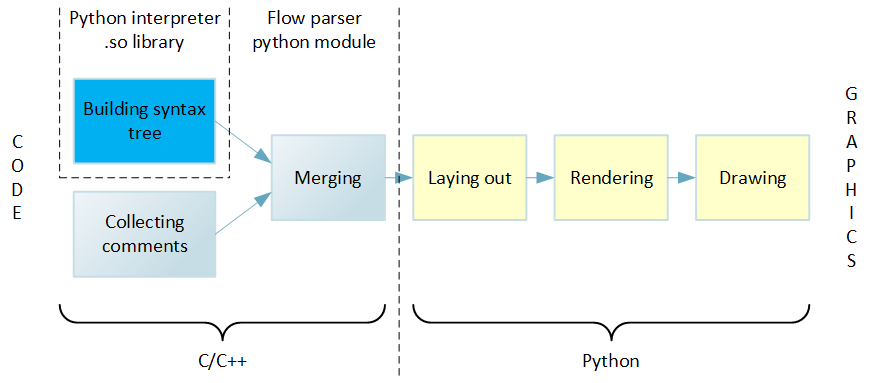
Code to Graphics Pipeline
Work begins with building a syntax tree from the source text. Then the tree is bypassed, and all detected blocks of code, loops, functions, etc. decomposed into a hierarchical data structure. After that, another pass is made through the source code, as a result of which information about the comments is collected. At further stages of the pipeline, it is more convenient to have comments already associated with recognized language constructs, rather than as separate data. Therefore, the next step is to merge the comments with the hierarchical structure representing the code. The described actions are performed by the flow parser extension module, which is written in C / C ++ to achieve the best performance.
The subsequent steps are already implemented inside the IDE and written in Python. This provides greater ease of experimentation with rendering compared to a C ++ implementation.
First, in a data structure called a virtual canvas, graphic elements are placed in accordance with the data structure received from the expansion module. Then comes the rendering phase, the main task of which is to calculate the sizes of all graphic elements. Finally, all graphic elements are drawn properly.
We will discuss all these stages in detail.
This is the very first stage on the way from text to graphics. Its task is to parse the source text and compose a hierarchical data structure. This is conveniently done using a syntax tree built from the source code. Obviously, I did not want to develop a new Python parser specifically for the project, but on the contrary, there was a desire to use something already ready. Fortunately, a suitable function was found right in the Python interpreter shared library. This C is a function that builds a tree in memory for the specified code. To visualize the work of this function, a utility was written that visually shows the constructed tree. For example, for the source text:
Such a tree will be built (for brevity, only a fragment is given):
In the output, each line corresponds to a tree node, nesting is shown by indentation, and for nodes all available information is shown.
In general, the tree looks very good: there is information about the row and column, there is a type of each node that corresponds to the formal Python grammar. But there are also problems. Firstly, there were comments in the code, but there is no information about them in the tree. Secondly, the information about the line and column numbers for the encoding is not true. Thirdly, the name of the encoding has changed. There was latin-1 in the code, and the syntax tree reports iso-8859-1. In the case of multi-line string literals, there is also a problem: there is no information about line numbers in the tree. All these surprises should be taken into account in the code that traverses the tree. However, all the problems described are rather trifles, compared with the complexity of the whole parser.
The extension module defines the types that will be visible in the Python code in subsequent stages. Types correspond to all recognizable elements, for example Class, Import, Break, etc. In addition to the data-specific members and functions specific to each case, all of them are intended to describe an element in terms of fragments: where a piece of text begins and where it ends.
When traversing the tree, a hierarchical structure is formed, an instance of the ControlFlow class, in which all recognized elements are laid out in the necessary way.
Due to the fact that there was no information about the comments in the syntax tree (it is obvious that the interpreter does not need them), and they are needed to display the code without loss, we had to introduce an additional pass through the source code. For this passage, information about each line of the comment is retrieved. This is easy to do, thanks to the simple Python grammar and the lack of multi-line comments as well as a preprocessor.
Comments are collected in the form of a list of fragments, where each fragment describes a single line of a comment by a set of attributes: line number, column number of the beginning and end, absolute positions in the file of the beginning and end of the comment.
For example, for the code:
Three fragments of the view will be collected:
When building a chart, it’s more convenient to deal not with two different data structures — executable code and comments — but with one. This simplifies the process of placing items on a virtual canvas. Therefore, another step is performed in the extension module: merging comments with recognized elements.
Consider an example:
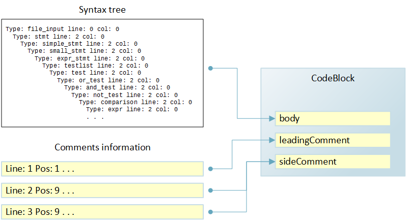
Merging comments with code
As a result of going through the syntax tree for the code above, an instance of the CodeBlock class will be generated. It, among other fields, has the body, leadingComment, and sideComment fields that describe the corresponding elements in terms of fragments. The body field will be populated with information from the syntax tree, and the comment fields will contain None.
Based on the results of the passage, a list of three fragments will be formed to collect comments. When merging, the first fragment will be used to populate the leadingComment field in the CodeBlock, and the second and third fragments for the sideComment field. Merging is based on line numbers available for both sources of information.
Thus, at the output of the merge stage, there is a completely ready-made single hierarchical data structure about the contents of a file or buffer in memory.
The pipeline stages described above are written in C / C ++ and are designed as a Python module. For general reasons, I wanted to make the work of all these stages quick in order to avoid unpleasant delays when redrawing diagrams during pauses for text modification. To test the performance, the module was launched on the existing platform:
to process all files of a standard Python installation 2.7.6. With 5707 files, processing took about 6 seconds. Of course, the files have different sizes and the module’s operating time depends on it, but the average result of about 1 millisecond per file is not on the fastest equipment, it seems to me more than acceptable. In practice, the text that needs to be processed is most often already stored in memory and the time of disk operations is completely gone, which also positively affects performance.
The purpose of this stage of the pipeline is to place all the necessary elements on a virtual canvas, taking into account the interconnections between them. A virtual canvas can be imagined as a canvas with rectangular cells. The cell may be empty, may contain one graphic element or a nested virtual canvas. At this stage, only the relative positioning of the elements is important, not the exact dimensions.
At the same time, the canvas does not have a fixed size and can grow down and to the right as needed. This approach corresponds to the prepared data structure and the method of drawing the chart. The process begins in the upper left corner. New rows and columns are added as needed. For example, a new line will be added for the next block of code, and if the block has a side comment, then a new column.
The set of graphic elements that can be placed in cells approximately corresponds to recognizable elements of the language with a small extension. For example, in the cell you may need a connector that leads from top to bottom, but in the language such an element is missing.
For a virtual canvas, a list of lists (two-dimensional array) is used, which is empty at the beginning of the process.
Consider a simple example to illustrate the process.
Placing graphic elements on the canvas The
left side of the image above shows the data structure generated by the results of code analysis. A ControlFlow instance contains several attributes and a suite container, in which there is only one element - a CodeBlock instance.
In the initial state, the canvas is empty, and the bypass of ControlFlow begins. The module was decided to draw as a scope, i.e. like a rounded rectangle. For the convenience of subsequent calculations of the sizes of graphic elements, taking into account the indentation, the rectangle of the visibility region is conditionally divided into components: faces and angles. The upper left corner of the rectangle of the module will be in the very top corner of the diagram, so we add a new line to the canvas, and add one column to the line and put an element in the scope corner cell. The upper edge of the rectangle can not be placed to the right, since the vertical margin is already at the expense of the first cell, and the rectangle will still be drawn as a single figure at the moment when the corner corner is detected at the stage of traversing the canvas.
Go to the next line. The module has a header that indicates the launch string and encoding. The values of the corresponding fields are None, but the title still needs to be drawn. Therefore, add a new line to the canvas. On the chart, the title should be inside the rectangle with a slight indent, so you can’t immediately place the title in the created line. In the first cell, the left face and then the title should be placed. Therefore, we add two columns and in the first we place scope left, and in the second - scope header. It is not necessary to place the right face in the third cell. Firstly, it is still unknown how many columns will be in the widest row. And secondly, the rectangle of the scope will still be drawn as a whole at the moment the corner corner is detected.
A module could have a documentation line, and it would need another line. But there is no documentation line, so go to suite. The first element in the suite is a block of code. We add a new row, and in it we add a column for the left face. Then we add one more column and place the graphic element for the code block in the cell. In the example, the block has a side comment, which should be located on the right, so we add another column and place a side comment in the cell.
There are no more elements in the suite, so the process of preparing a virtual canvas ends. The bottom left corner of the rectangle and the bottom face can not be added for reasons similar to those described above for the top and right sides. It is only necessary to take into account what they are meant when calculating the geometric dimensions of graphic elements.
The task of this stage of the pipeline is to calculate the sizes of all graphic primitives for drawing on the screen. This is done by traversing all placed cells, calculating the required sizes and saving them in the cell attributes.
Each cell has two calculated widths and two heights - the minimum necessary and actually required, taking into account the sizes of neighboring cells.
First, discuss how the height is calculated. This happens line by line. Consider the line that contains the elements corresponding to the assignment operator. Here you can see that the assignment operator occupies one text line, and the comment takes two. This means that the comment cell will require more vertical pixels on the screen when rendering. On the other hand, all cells in the row must be of the same height, otherwise the cells below will be drawn with an offset. This implies a simple algorithm. It is necessary to go around all the cells in the row and calculate for each the minimum height. Then select the maximum value from the just calculated and save it as the actual required height.
A bit more complicated is the situation with the calculation of the width of the cells. From this point of view, there are two types of strings:
A good example of dependent strings is the if statement. The branch that will be drawn under the condition block can be of arbitrary complexity, and therefore of arbitrary width. And the second branch, which should be drawn to the right, has a connector from the condition block located in the line above. This means that the width of the connector cell must be calculated depending on the lines below.
Thus, for independent rows, the width is calculated in one pass and the minimum width is the same as the actual one.
For regions of dependent strings, the algorithm is more complicated. First, the minimum widths of all cells in the region are calculated. And then, for each column, the actual width is calculated as the maximum value of the minimum required width for all cells in the region column. That is, it is very similar to what was done to calculate the height in the line.
Computations are done recursively for nested virtual canvases. The calculations take into account various settings: the metric of the selected font, fields for different cells, text indents, etc. Upon completion of the phase, everything necessary has already been prepared for placing graphic primitives already on the screen canvas.
The stage of drawing is very simple. Since the QT library is used for the user interface, a graphic scene is created with the dimensions calculated in the previous step. Then a recursive tour of the virtual canvas is carried out and the necessary elements with the necessary coordinates are added to the graphic scene.
The traversal process starts from the upper left corner and the current coordinates are set to 0, 0. Then the line is bypassed, after processing each cell, the width is added to the current x coordinate. When moving to the next line, the x coordinate is reset to 0, and the height of the line just processed is added to the y coordinate.
This completes the process of obtaining graphics by code.
We now discuss the functionality that has already been implemented and what can be added in the future.
The list of what has been done is quite short:
The combined use of already implemented individual changes of primitives, as practice shows, can significantly change the appearance of the diagram.
The possibilities that can complement the existing framework are limited only by imagination. The most obvious are listed here.
The features listed in the previous section can be divided into two groups:
For example, the scaling functionality is completely independent of the code. The current scale should rather be saved as the current IDE setting.
On the other hand, if branch switching is associated with a specific operator, and information on this should be somehow saved. After all, at the next session, if should be drawn as it was prescribed before.
Obviously, there are two ways to save additional information: either directly in the source text, or in a separate file, or even in many files. When making the decision, the following considerations were taken into account:
Thus, if there is a compact solution for saving additional information directly in files with the source text, then it is better to use it. Such a solution was found and was called CML: Codimension markup language.
CML is a micro markup language using python comments. Each CML comment consists of one or more adjacent lines. The format of the first line is selected as follows:
And the format of the continuation lines is as follows:
The literals cml and cml + are what distinguish CML comments from others. The version, which is an integer, has been introduced for the future if CML evolves. The type determines how the comment will affect the chart. The type used is a string identifier, for example rt (short for replace text). And key = value pairs provide an opportunity to describe all the necessary parameters.
As you can see, the format is simple and easy to read by humans. Thus, the requirement of the possibility of extracting additional useful information is satisfied not only when using the IDE, but also when viewing the text. Moreover, the only voluntary agreement between those who use and do not use graphics is this: do not break the CML comments.
Recognizing CML comments for replacing text is already implemented. It may appear as a leading comment before the block, for example:

Code block with modified text
No support from the GUI yet. You can add such a comment now only from a text editor. The purpose of the text parameter is quite obvious, and the rt type is chosen based on the abbreviation of replace text.
Recognizing CML comments for switching if branches is also already implemented. Support is both from the side of the text, and from the side of graphics. If you select a comment from the context menu of the condition block, the comment will be inserted in the right place in the code, and then the chart will be generated again.
If statement with the N branch to the right
In the above example, the N branch is drawn to the right of the condition.
It can be seen that this CML comment does not require any parameters. And its type sw is selected based on the abbreviation of the word switch.
Recognition of CML comments for color changing is already implemented. It may appear as a leading comment before the block, for example:

Block with individual colors.
Support for changing the color for the background (background parameter), font color (foreground parameter) and face color (border parameter). The cc type is selected based on the abbreviation of the words custom colors.
There is no support from the GUI yet. You can add such a comment now only from a text editor.
There is no support for this type of comment now, but it is already clear how the functionality can be implemented.
The sequence of actions may be as follows. The user selects a group of blocks on the diagram, taking into account the restrictions: the group has one input and one output. Next, from the context menu, select the item: combine into a group. The user then enters a title for the block to be drawn instead of the group. At the end of the input, the chart is redrawn in an updated form.
Obviously, for a group as a single entity, there are points in the code where it begins and where it ends. This means that you can insert CML comments in these places, for example, these:
Here, the uuid parameter is automatically generated at the time of the creation of the group and it is needed in order to correctly find pairs of the beginning of the group and its end, since there can be any number of nesting levels. The purpose of the title parameter is obvious - this is the text entered by the user. The record types gb and ge were introduced for the sake of abbreviations for the words group begin and group end, respectively.
Having uuid also allows you to diagnose various errors. For example, as a result of editing the text, one of the pair of CML comments could be deleted. Another case of the possible use of uuid is storing in the IDE groups, which should be shown as minimized in the next session.
The practice of using the tool showed that the technology has interesting side effects that were completely not considered during the initial development.
Firstly, it turned out to be convenient to use the generated diagrams for documentation and for discussion with colleagues, often not related to programming, but who are experts in the subject area. In such cases, code was prepared that was not intended to be executed, but corresponding to the logic of actions and corresponding to the formal syntax of python. The generated chart was either inserted into the documentation or printed and discussed. An additional convenience was manifested in the ease of making changes to the logic - the chart is instantly redrawn with all the necessary indents and aligned without the need for manual operations with graphics.
Secondly, an interesting purely psychological effect was manifested. The developer, opening his own long-written code using Codimension, noticed that the diagram looks ugly - too complicated or confusing. And in order to get a more elegant diagram, he made changes to the text, actually performing refactoring and simplification of the code. Which in turn leads to a decrease in the complexity of understanding and further support of the code.
Thirdly, despite the fact that the development was done for Python, the technology could well be extended to other programming languages. Python was chosen as a testing ground for several reasons: the language is popular, but at the same time syntactically simple.
I would like to thank everyone who helped in the work on this project. Thanks to my colleagues Dmitry Kazimirov, Ilya Loginov, David Makelhani and Sergey Fukanchik for their help with various aspects of development at different stages.
Special thanks to the authors and developers of the Python open source packages that were used in the work on the Codimension IDE.
Environment that supports graphical representation of code
In the second part, we will focus on the implementation, performed mainly on Python. Implemented and planned functionality, as well as the proposed micro markup language, will be discussed.
general information
The technology was implemented as part of an open source project called Codimension . All source code is available under the GPL v.3 license and is hosted in three repositories on github : two Python extension modules cdm-pythonparser and cdm-flowparser plus the IDE itself . The extension modules are mainly written in C / C ++, and the IDE in Python series 2. For the graphic part, the Python wrapper of the QT library - PyQT was used.
Development is done on Linux and for Linux. The main distribution used was Ubuntu.
The environment is designed to work with projects written in Python series 2.
Architecture
The diagram below shows the IDE architecture.
Architecture IDE
Blue on the diagram indicates the parts developed in the project. Yellow - third-party Python modules, and green - third-party binary modules.
From the very beginning of the project, it was obvious that it was completely impossible for one developer to develop all the required components from scratch in a reasonable amount of time. Therefore, the existing Python packages were used wherever possible and reasonable. The above diagram perfectly reflects the decision.
Only three parts are developed as part of the project. The IDE is written in Python to speed up development and simplify experimentation. Extension modules are written in C / C ++ for better responsiveness of the IDE. The task of brief parser is to report all entities found in the Python file (or buffer), such as imports, classes, functions, global variables, documentation lines, etc. The presence of such information allows you to implement, for example, such functionality: it is structured to show the contents of the file and provide navigation, provide an analysis of certain, but never used, functions, classes and global variables in the project. The task of flow parser is to provide in a convenient form the data necessary for drawing a chart.
All other components are third-party. PyQT was used for the interface and network part. QScintilla as the main text editor and some other elements, such as redirected input / output of debugged scripts or showing the svn version of a file of a specific revision. Graphviz was used to calculate the location of graphic elements in a dependency diagram, etc. Other ready-made Python packages were also used: pyflakes, pylint, filemagic, rope, gprof2dot, etc.
Code to Graphics Pipeline
The implementation of the transition from text to graphics is built on the principle of a pipeline. At each stage, a certain part of the work is performed, and the results are transferred to the next stage. The diagram below shows all stages of the pipeline, on the left of which the source text is input, and on the right at the output, a drawn diagram is obtained.
Code to Graphics Pipeline
Work begins with building a syntax tree from the source text. Then the tree is bypassed, and all detected blocks of code, loops, functions, etc. decomposed into a hierarchical data structure. After that, another pass is made through the source code, as a result of which information about the comments is collected. At further stages of the pipeline, it is more convenient to have comments already associated with recognized language constructs, rather than as separate data. Therefore, the next step is to merge the comments with the hierarchical structure representing the code. The described actions are performed by the flow parser extension module, which is written in C / C ++ to achieve the best performance.
The subsequent steps are already implemented inside the IDE and written in Python. This provides greater ease of experimentation with rendering compared to a C ++ implementation.
First, in a data structure called a virtual canvas, graphic elements are placed in accordance with the data structure received from the expansion module. Then comes the rendering phase, the main task of which is to calculate the sizes of all graphic elements. Finally, all graphic elements are drawn properly.
We will discuss all these stages in detail.
Building a syntax tree
This is the very first stage on the way from text to graphics. Its task is to parse the source text and compose a hierarchical data structure. This is conveniently done using a syntax tree built from the source code. Obviously, I did not want to develop a new Python parser specifically for the project, but on the contrary, there was a desire to use something already ready. Fortunately, a suitable function was found right in the Python interpreter shared library. This C is a function that builds a tree in memory for the specified code. To visualize the work of this function, a utility was written that visually shows the constructed tree. For example, for the source text:
#!/bin/env python
# encoding: latin-1
def f():
    # What printed?
    print 154
Such a tree will be built (for brevity, only a fragment is given):
$ ./tree test.py
Type: encoding_decl line: 0 col: 0 str: iso-8859-1
  Type: file_input line: 0 col: 0
    Type: stmt line: 4 col: 0
      Type: compound_stmt line: 4 col: 0
        Type: funcdef line: 4 col: 0
          Type: NAME line: 4 col: 0 str: def
          Type: NAME line: 4 col: 4 str: f
          Type: parameters line: 4 col: 5
            Type: LPAR line: 4 col: 5 str: (
            Type: RPAR line: 4 col: 6 str:)
          Type: COLON line: 4 col: 7 str::
          Type: suite line: 4 col: 8
            Type: NEWLINE line: 4 col: 8 str:
            Type: INDENT line: 6 col: -1 str:
            Type: stmt line: 6 col: 4
              Type: simple_stmt line: 6 col: 4
                Type: small_stmt line: 6 col: 4
                  Type: print_stmt line: 6 col: 4
                  . . .
In the output, each line corresponds to a tree node, nesting is shown by indentation, and for nodes all available information is shown.
In general, the tree looks very good: there is information about the row and column, there is a type of each node that corresponds to the formal Python grammar. But there are also problems. Firstly, there were comments in the code, but there is no information about them in the tree. Secondly, the information about the line and column numbers for the encoding is not true. Thirdly, the name of the encoding has changed. There was latin-1 in the code, and the syntax tree reports iso-8859-1. In the case of multi-line string literals, there is also a problem: there is no information about line numbers in the tree. All these surprises should be taken into account in the code that traverses the tree. However, all the problems described are rather trifles, compared with the complexity of the whole parser.
The extension module defines the types that will be visible in the Python code in subsequent stages. Types correspond to all recognizable elements, for example Class, Import, Break, etc. In addition to the data-specific members and functions specific to each case, all of them are intended to describe an element in terms of fragments: where a piece of text begins and where it ends.
When traversing the tree, a hierarchical structure is formed, an instance of the ControlFlow class, in which all recognized elements are laid out in the necessary way.
Comment collection
Due to the fact that there was no information about the comments in the syntax tree (it is obvious that the interpreter does not need them), and they are needed to display the code without loss, we had to introduce an additional pass through the source code. For this passage, information about each line of the comment is retrieved. This is easy to do, thanks to the simple Python grammar and the lack of multi-line comments as well as a preprocessor.
Comments are collected in the form of a list of fragments, where each fragment describes a single line of a comment by a set of attributes: line number, column number of the beginning and end, absolute positions in the file of the beginning and end of the comment.
For example, for the code:
#!/bin/env python
# encoding: latin-1
def f():
    # What printed?
    print 154
Three fragments of the view will be collected:
Line: 1 Pos: 1 ...
Line: 2 Pos: 1 ...
Line: 5 Pos: 5 ...
Merging comments with code snippets
When building a chart, it’s more convenient to deal not with two different data structures — executable code and comments — but with one. This simplifies the process of placing items on a virtual canvas. Therefore, another step is performed in the extension module: merging comments with recognized elements.
Consider an example:
# leading comment
a = 10  # side comment 1
        # side comment 2
Merging comments with code
As a result of going through the syntax tree for the code above, an instance of the CodeBlock class will be generated. It, among other fields, has the body, leadingComment, and sideComment fields that describe the corresponding elements in terms of fragments. The body field will be populated with information from the syntax tree, and the comment fields will contain None.
Based on the results of the passage, a list of three fragments will be formed to collect comments. When merging, the first fragment will be used to populate the leadingComment field in the CodeBlock, and the second and third fragments for the sideComment field. Merging is based on line numbers available for both sources of information.
Thus, at the output of the merge stage, there is a completely ready-made single hierarchical data structure about the contents of a file or buffer in memory.
Module performance
The pipeline stages described above are written in C / C ++ and are designed as a Python module. For general reasons, I wanted to make the work of all these stages quick in order to avoid unpleasant delays when redrawing diagrams during pauses for text modification. To test the performance, the module was launched on the existing platform:
- Intel Core i5-3210M laptop
- Ubuntu 14.04 LTS
to process all files of a standard Python installation 2.7.6. With 5707 files, processing took about 6 seconds. Of course, the files have different sizes and the module’s operating time depends on it, but the average result of about 1 millisecond per file is not on the fastest equipment, it seems to me more than acceptable. In practice, the text that needs to be processed is most often already stored in memory and the time of disk operations is completely gone, which also positively affects performance.
Placement on a virtual canvas
The purpose of this stage of the pipeline is to place all the necessary elements on a virtual canvas, taking into account the interconnections between them. A virtual canvas can be imagined as a canvas with rectangular cells. The cell may be empty, may contain one graphic element or a nested virtual canvas. At this stage, only the relative positioning of the elements is important, not the exact dimensions.
At the same time, the canvas does not have a fixed size and can grow down and to the right as needed. This approach corresponds to the prepared data structure and the method of drawing the chart. The process begins in the upper left corner. New rows and columns are added as needed. For example, a new line will be added for the next block of code, and if the block has a side comment, then a new column.
The set of graphic elements that can be placed in cells approximately corresponds to recognizable elements of the language with a small extension. For example, in the cell you may need a connector that leads from top to bottom, but in the language such an element is missing.
For a virtual canvas, a list of lists (two-dimensional array) is used, which is empty at the beginning of the process.
Consider a simple example to illustrate the process.
a = 10    # side comment 1
          # side comment 2
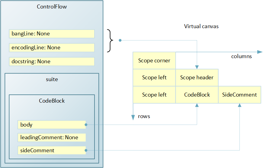
Placing graphic elements on the canvas The
left side of the image above shows the data structure generated by the results of code analysis. A ControlFlow instance contains several attributes and a suite container, in which there is only one element - a CodeBlock instance.
In the initial state, the canvas is empty, and the bypass of ControlFlow begins. The module was decided to draw as a scope, i.e. like a rounded rectangle. For the convenience of subsequent calculations of the sizes of graphic elements, taking into account the indentation, the rectangle of the visibility region is conditionally divided into components: faces and angles. The upper left corner of the rectangle of the module will be in the very top corner of the diagram, so we add a new line to the canvas, and add one column to the line and put an element in the scope corner cell. The upper edge of the rectangle can not be placed to the right, since the vertical margin is already at the expense of the first cell, and the rectangle will still be drawn as a single figure at the moment when the corner corner is detected at the stage of traversing the canvas.
Go to the next line. The module has a header that indicates the launch string and encoding. The values of the corresponding fields are None, but the title still needs to be drawn. Therefore, add a new line to the canvas. On the chart, the title should be inside the rectangle with a slight indent, so you can’t immediately place the title in the created line. In the first cell, the left face and then the title should be placed. Therefore, we add two columns and in the first we place scope left, and in the second - scope header. It is not necessary to place the right face in the third cell. Firstly, it is still unknown how many columns will be in the widest row. And secondly, the rectangle of the scope will still be drawn as a whole at the moment the corner corner is detected.
A module could have a documentation line, and it would need another line. But there is no documentation line, so go to suite. The first element in the suite is a block of code. We add a new row, and in it we add a column for the left face. Then we add one more column and place the graphic element for the code block in the cell. In the example, the block has a side comment, which should be located on the right, so we add another column and place a side comment in the cell.
There are no more elements in the suite, so the process of preparing a virtual canvas ends. The bottom left corner of the rectangle and the bottom face can not be added for reasons similar to those described above for the top and right sides. It is only necessary to take into account what they are meant when calculating the geometric dimensions of graphic elements.
Rendering
The task of this stage of the pipeline is to calculate the sizes of all graphic primitives for drawing on the screen. This is done by traversing all placed cells, calculating the required sizes and saving them in the cell attributes.
Each cell has two calculated widths and two heights - the minimum necessary and actually required, taking into account the sizes of neighboring cells.
First, discuss how the height is calculated. This happens line by line. Consider the line that contains the elements corresponding to the assignment operator. Here you can see that the assignment operator occupies one text line, and the comment takes two. This means that the comment cell will require more vertical pixels on the screen when rendering. On the other hand, all cells in the row must be of the same height, otherwise the cells below will be drawn with an offset. This implies a simple algorithm. It is necessary to go around all the cells in the row and calculate for each the minimum height. Then select the maximum value from the just calculated and save it as the actual required height.
A bit more complicated is the situation with the calculation of the width of the cells. From this point of view, there are two types of strings:
- those for which the width should be calculated taking into account the width of the cells in the adjacent row
- those whose cell widths can be calculated without regard to adjacent rows
A good example of dependent strings is the if statement. The branch that will be drawn under the condition block can be of arbitrary complexity, and therefore of arbitrary width. And the second branch, which should be drawn to the right, has a connector from the condition block located in the line above. This means that the width of the connector cell must be calculated depending on the lines below.
Thus, for independent rows, the width is calculated in one pass and the minimum width is the same as the actual one.
For regions of dependent strings, the algorithm is more complicated. First, the minimum widths of all cells in the region are calculated. And then, for each column, the actual width is calculated as the maximum value of the minimum required width for all cells in the region column. That is, it is very similar to what was done to calculate the height in the line.
Computations are done recursively for nested virtual canvases. The calculations take into account various settings: the metric of the selected font, fields for different cells, text indents, etc. Upon completion of the phase, everything necessary has already been prepared for placing graphic primitives already on the screen canvas.
Painting
The stage of drawing is very simple. Since the QT library is used for the user interface, a graphic scene is created with the dimensions calculated in the previous step. Then a recursive tour of the virtual canvas is carried out and the necessary elements with the necessary coordinates are added to the graphic scene.
The traversal process starts from the upper left corner and the current coordinates are set to 0, 0. Then the line is bypassed, after processing each cell, the width is added to the current x coordinate. When moving to the next line, the x coordinate is reset to 0, and the height of the line just processed is added to the y coordinate.
This completes the process of obtaining graphics by code.
Present and future
We now discuss the functionality that has already been implemented and what can be added in the future.
The list of what has been done is quite short:
- Automatic chart update in pauses of code change.
- Manual synchronization of visible text and graphics in both directions. If the input focus is in a text editor and a special key combination is pressed, then the diagram searches for the primitive that most closely matches the current cursor position. Next, the primitive is highlighted, and the chart scrolls to make the primitive visible. In the opposite direction, synchronization is performed by double-clicking on the primitive, which leads to moving the text cursor to the desired line of code and scrolling through the text editor, if necessary.
- Scaling chart. The current implementation uses built-in QT library scaling tools. In the future, it is planned to replace it with scaling by changing the font size and recalculating the sizes of all elements.
- Export charts to PDF, PNG and SVG. The quality of the output documents is determined by the implementation of the QT library, since it is precisely its tools that were used for this functionality.
- Scope navigation pane. Graphics make heavy use of the idea of scope, so a typical diagram contains many nested areas. The navigation bar shows the current path in terms of nested scopes for the current position of the mouse cursor over the graphics scene.
- Individual switching of branches for the if statement. By default, the N branch is drawn below, and the Y branch to the right. The diagram allows you to swap the location of branches using the context menu of the condition block.
- Individual replacement of the text of any graphic primitive. Sometimes there is a desire to replace the text of a block with an arbitrary one. For example, a condition in terms of variables and function calls can be long and not at all obvious, while a phrase in a natural language can better describe what is happening. The chart allows you to replace the displayed text with any one and shows the source in a tooltip.
- Individual replacement of colors of any primitive. Sometimes there is a desire to draw attention to any part of the code by highlighting graphic primitives. For example, a potentially dangerous area can be highlighted in red or a common color can be selected for elements responsible for overall functionality. The diagram allows you to change the background color, font and stroke of primitives.
The combined use of already implemented individual changes of primitives, as practice shows, can significantly change the appearance of the diagram.
The possibilities that can complement the existing framework are limited only by imagination. The most obvious are listed here.
- Automatic synchronization of text and graphics when scrolling.
- Support for editing on a chart: deleting, moving and adding blocks. Editing text inside individual blocks. Copy and paste blocks.
- Support for group operations with blocks.
- Visualization of debugging on a chart. At least the highlight of the current block and the current line in it.
- Support chart search.
- Print support.
- Management of hiding / showing various elements: comments, documentation lines, function bodies, classes, loops, etc.
- Highlighting of various types of imports: within the project, system, unidentified.
- Support for additional non-language blocks or pictures on diagrams.
- Smart scaling. You can enter several fixed levels of scale: all elements, without comments and documentation lines, only class and function headers, dependencies between files in a subdirectory, and pointers to external links. If you fix this behavior to the mouse wheel with any modifier, then you can get overview information extremely quickly.
- Roll up multiple blocks into one and roll back. A group of blocks performing a joint task can be selected on the diagram and collapsed into one block with its own graphics and provided text. The natural limitation here is that a group must have one input and one output. Such functionality may come in handy when working with unknown code. When it comes to understanding that several arranged blocks do, you can reduce the complexity of the diagram by combining the group and replacing it with one block with the desired signature, for example, “MD5 calculation”. Of course, at any time it will be possible to return to the details. This function can be considered as the introduction of the third dimension in the diagram.
CML v.1
The features listed in the previous section can be divided into two groups:
- Requiring the preservation of information in connection with the code.
- Completely code independent.
For example, the scaling functionality is completely independent of the code. The current scale should rather be saved as the current IDE setting.
On the other hand, if branch switching is associated with a specific operator, and information on this should be somehow saved. After all, at the next session, if should be drawn as it was prescribed before.
Obviously, there are two ways to save additional information: either directly in the source text, or in a separate file, or even in many files. When making the decision, the following considerations were taken into account:
- Imagine that a team of developers is working on a project and some of them are successfully using the graphical capabilities of the code presentation. And the other part of the fundamental considerations for working with code uses only vim. In this case, if additional information is stored separately from the code, then its consistency during alternate code editing by members of different camps will be extremely difficult, if not impossible, to support. Surely the additional information will turn out to be untrue at some point in time.
- If the approach of additional files is chosen, then they rather litter the contents of the project and require additional efforts from the team when working with version control systems.
- When a developer introduces additional markup - for example, replaces a long code of an incomprehensible condition with a suitable phrase - this is not for fun, but because such a markup is valuable. It would be nice to keep this value available for those who do not use the graphics, even if not in such a beautiful form.
Thus, if there is a compact solution for saving additional information directly in files with the source text, then it is better to use it. Such a solution was found and was called CML: Codimension markup language.
CML is a micro markup language using python comments. Each CML comment consists of one or more adjacent lines. The format of the first line is selected as follows:
# cml <версия> <тип> [пары ключ=значение]And the format of the continuation lines is as follows:
# cml+ <продолжение предыдущей cml строки>The literals cml and cml + are what distinguish CML comments from others. The version, which is an integer, has been introduced for the future if CML evolves. The type determines how the comment will affect the chart. The type used is a string identifier, for example rt (short for replace text). And key = value pairs provide an opportunity to describe all the necessary parameters.
As you can see, the format is simple and easy to read by humans. Thus, the requirement of the possibility of extracting additional useful information is satisfied not only when using the IDE, but also when viewing the text. Moreover, the only voluntary agreement between those who use and do not use graphics is this: do not break the CML comments.
CML: text replacement
Recognizing CML comments for replacing text is already implemented. It may appear as a leading comment before the block, for example:
# cml 1 rt text="Believe me, I do the right thing here"
False = 154
Code block with modified text
No support from the GUI yet. You can add such a comment now only from a text editor. The purpose of the text parameter is quite obvious, and the rt type is chosen based on the abbreviation of replace text.
CML: if branch switching
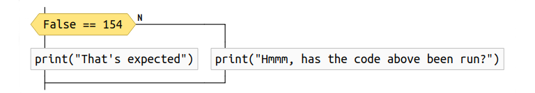
Recognizing CML comments for switching if branches is also already implemented. Support is both from the side of the text, and from the side of graphics. If you select a comment from the context menu of the condition block, the comment will be inserted in the right place in the code, and then the chart will be generated again.
# cml 1 sw
if False == 154:
    print("That’s expected")
else:
    print("Hmmm, has the code above been run?")
If statement with the N branch to the right
In the above example, the N branch is drawn to the right of the condition.
It can be seen that this CML comment does not require any parameters. And its type sw is selected based on the abbreviation of the word switch.
CML: color change
Recognition of CML comments for color changing is already implemented. It may appear as a leading comment before the block, for example:
# cml 1 cc background="255,138,128"
# cml+ foreground="0,0,255"
# cml+ border="0,0,0"
print("Danger! Someone has damaged False")
Block with individual colors.
Support for changing the color for the background (background parameter), font color (foreground parameter) and face color (border parameter). The cc type is selected based on the abbreviation of the words custom colors.
There is no support from the GUI yet. You can add such a comment now only from a text editor.
CML: group folding
There is no support for this type of comment now, but it is already clear how the functionality can be implemented.
The sequence of actions may be as follows. The user selects a group of blocks on the diagram, taking into account the restrictions: the group has one input and one output. Next, from the context menu, select the item: combine into a group. The user then enters a title for the block to be drawn instead of the group. At the end of the input, the chart is redrawn in an updated form.
Obviously, for a group as a single entity, there are points in the code where it begins and where it ends. This means that you can insert CML comments in these places, for example, these:
# cml gb uuid="..." title="..."
. . .
# cml ge uuid="..."
Here, the uuid parameter is automatically generated at the time of the creation of the group and it is needed in order to correctly find pairs of the beginning of the group and its end, since there can be any number of nesting levels. The purpose of the title parameter is obvious - this is the text entered by the user. The record types gb and ge were introduced for the sake of abbreviations for the words group begin and group end, respectively.
Having uuid also allows you to diagnose various errors. For example, as a result of editing the text, one of the pair of CML comments could be deleted. Another case of the possible use of uuid is storing in the IDE groups, which should be shown as minimized in the next session.
Side effects
The practice of using the tool showed that the technology has interesting side effects that were completely not considered during the initial development.
Firstly, it turned out to be convenient to use the generated diagrams for documentation and for discussion with colleagues, often not related to programming, but who are experts in the subject area. In such cases, code was prepared that was not intended to be executed, but corresponding to the logic of actions and corresponding to the formal syntax of python. The generated chart was either inserted into the documentation or printed and discussed. An additional convenience was manifested in the ease of making changes to the logic - the chart is instantly redrawn with all the necessary indents and aligned without the need for manual operations with graphics.
Secondly, an interesting purely psychological effect was manifested. The developer, opening his own long-written code using Codimension, noticed that the diagram looks ugly - too complicated or confusing. And in order to get a more elegant diagram, he made changes to the text, actually performing refactoring and simplification of the code. Which in turn leads to a decrease in the complexity of understanding and further support of the code.
Thirdly, despite the fact that the development was done for Python, the technology could well be extended to other programming languages. Python was chosen as a testing ground for several reasons: the language is popular, but at the same time syntactically simple.
Acknowledgments
I would like to thank everyone who helped in the work on this project. Thanks to my colleagues Dmitry Kazimirov, Ilya Loginov, David Makelhani and Sergey Fukanchik for their help with various aspects of development at different stages.
Special thanks to the authors and developers of the Python open source packages that were used in the work on the Codimension IDE.