A small study of the properties of a simple U-net, a classical convolutional network for segmentation
The article is written according to the analysis and study of materials for the competition to search for ships at sea.
Let's try to understand how and what the network is looking for and what it finds. This article is simply the result of curiosity and idle interest, nothing of it is encountered in practice, and for practical tasks there is nothing to copy and paste. But the result is not quite expected. The Internet is full of descriptions of the work of networks in which the authors beautifully and with pictures tell how networks determine primitives - corners, circles, whiskers, tails, etc., then they are searched for segmentation / classification. Many competitions are won using weights from other large and wide networks. It is interesting to understand and see how and what primitives the network builds.
Let's do a little research and consider the options - the author's reasoning and the code are set out, you can check / add / change everything yourself.
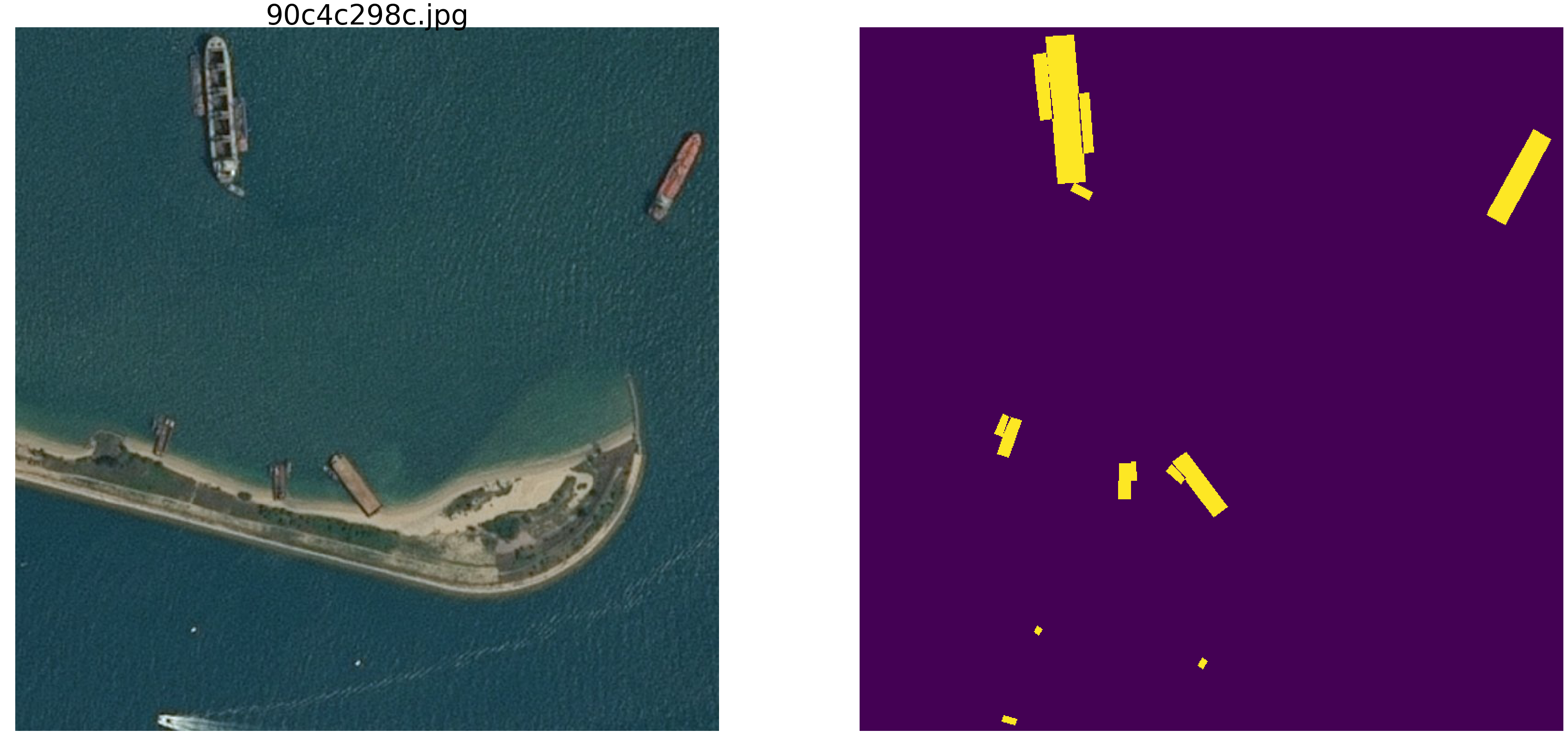
Recently ended kaggle competition for finding ships at sea. Airbus offered to analyze satellite images of the sea, both with and without vessels. A total of 192555 768x768x3 pictures is 340 720 680 960 bytes if uint8 and four times as many if float32 (by the way float32 is faster than float64, fewer memory accesses) and you need to find ships in 15606 pictures. As usual, all significant places were taken by people involved in ODS (ods.ai), which is natural and expected, and I hope that we will soon be able to study the train of thought and the code of winners and prize-winners.
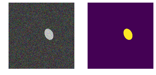
We will consider a similar task, but we will simplify it significantly - take the sea np.random.sample * 0.5, we do not need waves, wind, shores and other hidden patterns and faces. Let's make the image of the sea really random in the RGB range from 0.0 to 0.5. We will color the vessels in the same color and in order to distinguish them from the sea, we will place them in the range from 0.5 to 1.0, and they will all be of the same shape - ellipses of different sizes and orientations.
Take a very common version of the network (you can take your favorite network) and all the experiments we will do with it.
Next, we will change the parameters of the image, interfere with and build hypotheses - so we select the main features by which the network finds ellipses. Perhaps the reader will make his conclusions and the author will refute.
We use the classic metric in image segmentation, there are a lot of articles, a code with comments and a text about the selected metric, on the same kaggle there are a lot of options with comments and explanations. We will predict the pixel mask - this is the "sea" or "ship" and evaluate the truth or falsehood of the prediction. Those. the following four options are possible - we correctly predicted that a pixel is a “sea”, correctly predicted that a pixel is a “ship” or made a mistake in predicting a “sea” or “ship”. And so on all the pictures and all the pixels we estimate the number of all four options and calculate the result - this will be the result of the network. And the fewer erroneous predictions and the more true, the more accurate the result and the better the operation of the network.
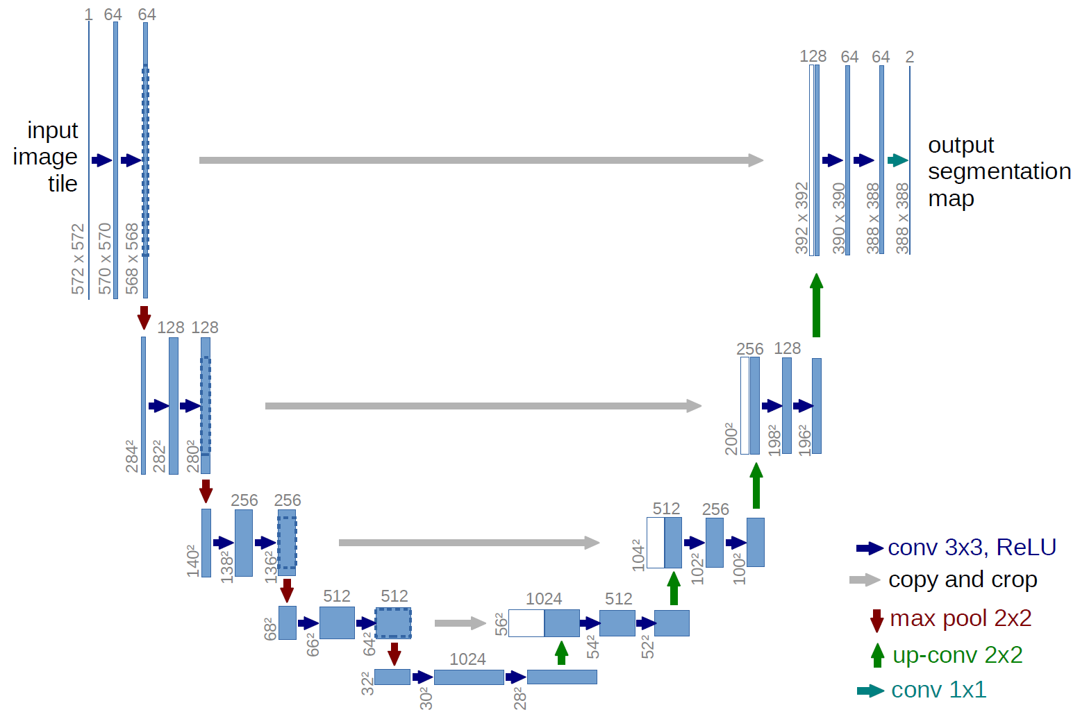
And for research we will take a well-studied u-net, this is an excellent network for image segmentation. The network is very common in such competitions and there are many descriptions, subtleties of application, etc. A variant of the classic U-net was chosen and, of course, it was possible to modernize it, add residual blocks, etc. But "it is impossible to embrace the immense" and conduct all the experiments and tests at once. U-net performs a very simple operation with pictures - step-by-step reduces the dimension of the picture with some transformations and afterwards tries to restore the mask from the compressed image. Those. the dimension of the picture in our case is brought to 32x32 and then we try to restore the mask using data from all previous compressions.
The picture shows the U-net scheme from the original article, but we have slightly altered it, but the essence remains the same - compress the image → expand it into the mask.
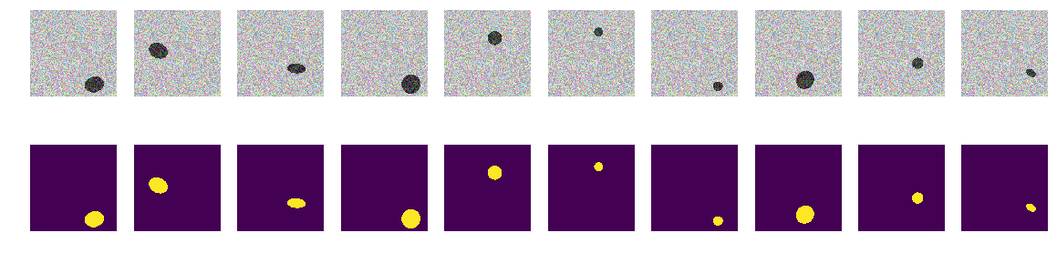
The first version of our experiment was chosen especially for clarity, very simple - the sea is lighter, the vessels are darker. Everything is very simple and obvious, we hypothesize that the network will find the ships / ellipses without problems and with any accuracy. The next_pair function generates a picture / mask pair in which the location, size, angle of rotation are chosen randomly. Further, all changes will be made to this function - changing the coloring, shape, noise, etc. But now the easiest option, check the hypothesis of dark ships on a light background.
We generate the whole train and see what happens. It is quite similar to the ships in the sea and nothing superfluous. Everything is clearly visible, clear and understandable. The arrangement is random, and there is only one ellipse in each picture.
There is no doubt that the network will learn successfully and will find ellipses. But let's check our hypothesis that the network is learning to find ellipses / ships and at the same time with high accuracy.
The net successfully finds ellipses. But it is not at all proven that it is looking for ellipses in the human understanding, as the area is bounded by the equation of the ellipse and filled with different content from the background, there is no certainty that there will be network weights similar to the coefficients of the quadratic equation of the ellipse. And it is obvious that the brightness of the ellipse is less than the brightness of the background and no secret and riddle - we assume that we just checked the code. Let's correct the obvious face, make the background and the color of the ellipse also random.
Now the same ellipses on the same sea, but the color of the sea and, accordingly, the ship is chosen randomly. If the sea is darker, the ship will be lighter and vice versa. Those. According to the brightness of the group of points, it is impossible to determine whether they are located outside the ellipse, i.e., the sea or it is the points inside the ellipse. And again we check our hypothesis that the network will find ellipses regardless of color.
Now it is impossible to determine the background or ellipse by pixel and its surroundings. We also generate images and masks and look at the first 10 on the screen.
The network easily copes and finds all ellipses. But even here there is a flaw in the implementation, and everything is obvious - the smaller of the two areas in the picture is the ellipse, another background. Perhaps this is an incorrect hypothesis, but still correct, add another polygon on the image of the same color as the ellipse.
On each picture, we randomly select the color of the sea from two options and add an ellipse and a rectangle both different from the color of the sea. It turns out the same "sea", just painted "ship", but in the same picture add a rectangle of the same color as the "ship" and also with a randomly selected size. Now our assumption is more complicated, in the picture there are two equally colored objects, but we hypothesize that the network will still learn to choose the right object.
Just as before, we calculate pictures and masks and look at the first 10 pairs.
It was not possible to confuse the network with rectangles and our hypothesis is confirmed. At the Airbus competition, everyone, judging by examples and discussions, was a single vessel, and several vessels were quite close by. Ellipse from the rectangle - i.e. the ship is different from the house on the shore, the network is different, although the polygons are of the same color as the ellipses. The point is not in color, because both the ellipse and the rectangle are equally randomly colored.
Perhaps the network is distinguished by rectangles - correct, distort them. Those. the network easily finds both closed areas regardless of shape and discards the one that is rectangle. This is the author's hypothesis - let's check it, for which we will add not rectangles, but quadrilateral polygons of arbitrary shape. And again our hypothesis is that the network will distinguish an ellipse from an arbitrary quadrilateral polygon of the same coloring.
You can certainly get into the inside of the network and look at the layers there and analyze the meaning of weights and shifts. The author is interested in the resulting behavior of the network, the judgment will be based on the result of the work, although it is always interesting to look inside.
We calculate pictures and masks and look at the first 10 pairs.
We start our network. Let me remind you that it is the same for all options.
The hypothesis is confirmed, polygons and ellipses are easily distinguishable. The attentive reader will note here - of course they are different, a nonsense question, any normal AI can distinguish a second-order curve from the first line. Those. the network easily determines the presence of a boundary in the form of a second order curve. We will not argue, replace the oval by the heptagon and check.
There are no curves, only flat faces of regular inclined and rotated heptagons and arbitrary quadrangular polygons. Let us change the image / mask generator to the change function - only the projections of regular hexagons and arbitrary quadrangular polygons of the same color.
Just as before we build arrays and look at the first 10.
As we can see, the network distinguishes the projections of regular heptagons and arbitrary quadrilateral polygons with an accuracy of 0.828 on the test set. Network training is stopped at an arbitrary value of 0.75 and most likely the accuracy should be much better. If we proceed from the thesis that the network finds primitives and their combinations define an object, then in our case there are two areas with their average differing from the background, there are no primitives in the understanding of man. There are no clear, monochromatic lines, and corners, respectively, not, only areas with very similar boundaries. Even if lines are drawn, then both objects in the picture are built from identical primitives.
A question for connoisseurs - what does the network consider to be a sign that distinguishes "ships" from "interference"? Obviously, this is not the color or shape of the borders of the ships. You can of course continue to continue the study of this abstract construction "sea" / "ships", we are not an Academy of Sciences and can conduct research solely out of curiosity. We can change heptagons to octagons or fill in a picture with regular five and six squares and see if the network will distinguish them or not. I leave it for the readers - although it also became interesting to me whether the network can count the number of corners of a polygon and, for a test, place in the picture not regular polygons, but their random projections.
There are other, no less interesting properties of such ships, and such experiments are useful in that we set all the probabilistic characteristics of the set under study and the unexpected behavior of well-studied networks will add knowledge and benefit.
The background is random, the color is random, the place of the ship / ellipse is random. There are no lines in the pictures, there are areas with different characteristics, but there are no monochrome lines! In this case, of course there are simplifications and the task can be complicated - for example, choosing colors like 0.0 ... 0.9 and 0.1 ... 1.0 - but there is no difference for the network. The network can and does find patterns that differ from those that a person clearly sees and finds.
If someone from the readers is interested, you can continue to research and tinkering in the networks, if something does not work or is not clear, or suddenly a new and good idea appears and amazes with its beauty, then you can always share with us or ask the masters (and grandmasters too) and ask for qualified help in the ODS community.
Let's try to understand how and what the network is looking for and what it finds. This article is simply the result of curiosity and idle interest, nothing of it is encountered in practice, and for practical tasks there is nothing to copy and paste. But the result is not quite expected. The Internet is full of descriptions of the work of networks in which the authors beautifully and with pictures tell how networks determine primitives - corners, circles, whiskers, tails, etc., then they are searched for segmentation / classification. Many competitions are won using weights from other large and wide networks. It is interesting to understand and see how and what primitives the network builds.
Let's do a little research and consider the options - the author's reasoning and the code are set out, you can check / add / change everything yourself.
Recently ended kaggle competition for finding ships at sea. Airbus offered to analyze satellite images of the sea, both with and without vessels. A total of 192555 768x768x3 pictures is 340 720 680 960 bytes if uint8 and four times as many if float32 (by the way float32 is faster than float64, fewer memory accesses) and you need to find ships in 15606 pictures. As usual, all significant places were taken by people involved in ODS (ods.ai), which is natural and expected, and I hope that we will soon be able to study the train of thought and the code of winners and prize-winners.
We will consider a similar task, but we will simplify it significantly - take the sea np.random.sample * 0.5, we do not need waves, wind, shores and other hidden patterns and faces. Let's make the image of the sea really random in the RGB range from 0.0 to 0.5. We will color the vessels in the same color and in order to distinguish them from the sea, we will place them in the range from 0.5 to 1.0, and they will all be of the same shape - ellipses of different sizes and orientations.
Take a very common version of the network (you can take your favorite network) and all the experiments we will do with it.
Next, we will change the parameters of the image, interfere with and build hypotheses - so we select the main features by which the network finds ellipses. Perhaps the reader will make his conclusions and the author will refute.
Load the library, determine the size of the array of images
import numpy as np
import pandas as pd
import matplotlib.pyplot as plt
%matplotlib inline
import math
from tqdm import tqdm_notebook, tqdm
from skimage.draw import ellipse, polygon
from keras import Model
from keras.callbacks import EarlyStopping, ModelCheckpoint, ReduceLROnPlateau
from keras.models import load_model
from keras.optimizers import Adam
from keras.layers import Input, Conv2D, Conv2DTranspose, MaxPooling2D, concatenate, Dropout
from keras.losses import binary_crossentropy
import tensorflow as tf
import keras as keras
from keras import backend as K
from tqdm import tqdm_notebook
w_size = 256
train_num = 8192
train_x = np.zeros((train_num, w_size, w_size,3), dtype='float32')
train_y = np.zeros((train_num, w_size, w_size,1), dtype='float32')
img_l = np.random.sample((w_size, w_size, 3))*0.5
img_h = np.random.sample((w_size, w_size, 3))*0.5 + 0.5
radius_min = 10
radius_max = 30
define loss and accuracy functions
defdice_coef(y_true, y_pred):
    y_true_f = K.flatten(y_true)
    y_pred = K.cast(y_pred, 'float32')
    y_pred_f = K.cast(K.greater(K.flatten(y_pred), 0.5), 'float32')
    intersection = y_true_f * y_pred_f
    score = 2. * K.sum(intersection) / (K.sum(y_true_f) + K.sum(y_pred_f))
    return score
defdice_loss(y_true, y_pred):
    smooth = 1.
    y_true_f = K.flatten(y_true)
    y_pred_f = K.flatten(y_pred)
    intersection = y_true_f * y_pred_f
    score = (2. * K.sum(intersection) + smooth) / (K.sum(y_true_f) + K.sum(y_pred_f) + smooth)
    return1. - score
defbce_dice_loss(y_true, y_pred):return binary_crossentropy(y_true, y_pred) + dice_loss(y_true, y_pred)
defget_iou_vector(A, B):# Numpy version
    batch_size = A.shape[0]
    metric = 0.0for batch in range(batch_size):
        t, p = A[batch], B[batch]
        true = np.sum(t)
        pred = np.sum(p)
        # deal with empty mask firstif true == 0:
            metric += (pred == 0)
            continue# non empty mask case.  Union is never empty # hence it is safe to divide by its number of pixels
        intersection = np.sum(t * p)
        union = true + pred - intersection
        iou = intersection / union
        # iou metrric is a stepwise approximation of the real iou over 0.5
        iou = np.floor(max(0, (iou - 0.45)*20)) / 10
        metric += iou
    # teake the average over all images in batch
    metric /= batch_size
    return metric
defmy_iou_metric(label, pred):# Tensorflow versionreturn tf.py_func(get_iou_vector, [label, pred > 0.5], tf.float64)
from keras.utils.generic_utils import get_custom_objects
get_custom_objects().update({'bce_dice_loss': bce_dice_loss })
get_custom_objects().update({'dice_loss': dice_loss })
get_custom_objects().update({'dice_coef': dice_coef })
get_custom_objects().update({'my_iou_metric': my_iou_metric })
We use the classic metric in image segmentation, there are a lot of articles, a code with comments and a text about the selected metric, on the same kaggle there are a lot of options with comments and explanations. We will predict the pixel mask - this is the "sea" or "ship" and evaluate the truth or falsehood of the prediction. Those. the following four options are possible - we correctly predicted that a pixel is a “sea”, correctly predicted that a pixel is a “ship” or made a mistake in predicting a “sea” or “ship”. And so on all the pictures and all the pixels we estimate the number of all four options and calculate the result - this will be the result of the network. And the fewer erroneous predictions and the more true, the more accurate the result and the better the operation of the network.
And for research we will take a well-studied u-net, this is an excellent network for image segmentation. The network is very common in such competitions and there are many descriptions, subtleties of application, etc. A variant of the classic U-net was chosen and, of course, it was possible to modernize it, add residual blocks, etc. But "it is impossible to embrace the immense" and conduct all the experiments and tests at once. U-net performs a very simple operation with pictures - step-by-step reduces the dimension of the picture with some transformations and afterwards tries to restore the mask from the compressed image. Those. the dimension of the picture in our case is brought to 32x32 and then we try to restore the mask using data from all previous compressions.
The picture shows the U-net scheme from the original article, but we have slightly altered it, but the essence remains the same - compress the image → expand it into the mask.
Just u-net
defbuild_model(input_layer, start_neurons):
    conv1 = Conv2D(start_neurons*1,(3,3),activation="relu", padding="same")(input_layer)
    conv1 = Conv2D(start_neurons*1,(3,3),activation="relu", padding="same")(conv1)
    pool1 = MaxPooling2D((2, 2))(conv1)
    pool1 = Dropout(0.25)(pool1)
    conv2 = Conv2D(start_neurons*2,(3,3),activation="relu", padding="same")(pool1)
    conv2 = Conv2D(start_neurons*2,(3,3),activation="relu", padding="same")(conv2)
    pool2 = MaxPooling2D((2, 2))(conv2)
    pool2 = Dropout(0.5)(pool2)
    conv3 = Conv2D(start_neurons*4,(3,3),activation="relu", padding="same")(pool2)
    conv3 = Conv2D(start_neurons*4,(3,3),activation="relu", padding="same")(conv3)
    pool3 = MaxPooling2D((2, 2))(conv3)
    pool3 = Dropout(0.5)(pool3)
    conv4 = Conv2D(start_neurons*8,(3,3),activation="relu", padding="same")(pool3)
    conv4 = Conv2D(start_neurons*8,(3,3),activation="relu", padding="same")(conv4)
    pool4 = MaxPooling2D((2, 2))(conv4)
    pool4 = Dropout(0.5)(pool4)
    # Middle
    convm = Conv2D(start_neurons*16,(3,3),activation="relu", padding="same")(pool4)
    convm = Conv2D(start_neurons*16,(3,3),activation="relu", padding="same")(convm)
    deconv4 = Conv2DTranspose(start_neurons * 8, (3, 3), strides=(2, 2), padding="same")(convm)
    uconv4 = concatenate([deconv4, conv4])
    uconv4 = Dropout(0.5)(uconv4)
    uconv4 = Conv2D(start_neurons*8,(3,3),activation="relu", padding="same")(uconv4)
    uconv4 = Conv2D(start_neurons*8,(3,3),activation="relu", padding="same")(uconv4)
    deconv3 = Conv2DTranspose(start_neurons*4,(3,3),strides=(2, 2), padding="same")(uconv4)
    uconv3 = concatenate([deconv3, conv3])
    uconv3 = Dropout(0.5)(uconv3)
    uconv3 = Conv2D(start_neurons*4,(3,3),activation="relu", padding="same")(uconv3)
    uconv3 = Conv2D(start_neurons*4,(3,3),activation="relu", padding="same")(uconv3)
    deconv2 = Conv2DTranspose(start_neurons*2,(3,3),strides=(2, 2), padding="same")(uconv3)
    uconv2 = concatenate([deconv2, conv2])
    uconv2 = Dropout(0.5)(uconv2)
    uconv2 = Conv2D(start_neurons*2,(3,3),activation="relu", padding="same")(uconv2)
    uconv2 = Conv2D(start_neurons*2,(3,3),activation="relu", padding="same")(uconv2)
    deconv1 = Conv2DTranspose(start_neurons*1,(3,3),strides=(2, 2), padding="same")(uconv2)
    uconv1 = concatenate([deconv1, conv1])
    uconv1 = Dropout(0.5)(uconv1)
    uconv1 = Conv2D(start_neurons*1,(3,3),activation="relu", padding="same")(uconv1)
    uconv1 = Conv2D(start_neurons*1,(3,3),activation="relu", padding="same")(uconv1)
    uncov1 = Dropout(0.5)(uconv1)
    output_layer = Conv2D(1,(1,1), padding="same", activation="sigmoid")(uconv1)
    return output_layer
The first experiment. Simplest
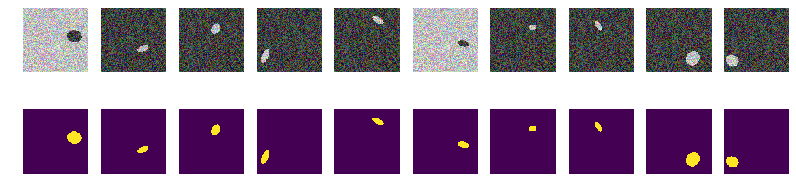
The first version of our experiment was chosen especially for clarity, very simple - the sea is lighter, the vessels are darker. Everything is very simple and obvious, we hypothesize that the network will find the ships / ellipses without problems and with any accuracy. The next_pair function generates a picture / mask pair in which the location, size, angle of rotation are chosen randomly. Further, all changes will be made to this function - changing the coloring, shape, noise, etc. But now the easiest option, check the hypothesis of dark ships on a light background.
defnext_pair():
    p = np.random.sample() - 0.5# пока не успользуем# r,c - координаты центра эллипса
    r = np.random.sample()*(w_size-2*radius_max) + radius_max
    c = np.random.sample()*(w_size-2*radius_max) + radius_max
    # большой и малый радиусы эллипса
    r_radius = np.random.sample()*(radius_max-radius_min) + radius_min
    c_radius = np.random.sample()*(radius_max-radius_min) + radius_min
    rot = np.random.sample()*360#  наклон эллипса
    rr, cc = ellipse(
      r, c,
      r_radius, c_radius,
      rotation=np.deg2rad(rot),
      shape=img_l.shape
    )  # получаем все точки эллипса# красим пиксели моря/фона в шум от 0.5 до 1.0
    img = img_h.copy()
    # красим пиксели эллипса в шум от 0.0  до 0.5
    img[rr, cc] = img_l[rr, cc]
    msk = np.zeros((w_size, w_size, 1), dtype='float32')
    msk[rr, cc] = 1.# красим пиксели маски эллипсаreturn img, msk
We generate the whole train and see what happens. It is quite similar to the ships in the sea and nothing superfluous. Everything is clearly visible, clear and understandable. The arrangement is random, and there is only one ellipse in each picture.
for k in range(train_num): # генерация всех img train
    img, msk = next_pair()
    train_x[k] = img
    train_y[k] = msk
fig, axes = plt.subplots(2, 10, figsize=(20, 5)) # смотрим на первые 10 с маскамиfor k in range(10):
    axes[0,k].set_axis_off()
    axes[0,k].imshow(train_x[k])
    axes[1,k].set_axis_off()
    axes[1,k].imshow(train_y[k].squeeze())
There is no doubt that the network will learn successfully and will find ellipses. But let's check our hypothesis that the network is learning to find ellipses / ships and at the same time with high accuracy.
input_layer = Input((w_size, w_size, 3))
output_layer = build_model(input_layer, 16)
model = Model(input_layer, output_layer)
model.compile(loss=bce_dice_loss, optimizer=Adam(lr=1e-3), metrics=[my_iou_metric])
model.save_weights('./keras.weights')
whileTrue:
    history = model.fit(train_x, train_y,
                        batch_size=32,
                        epochs=1,
                        verbose=1,
                        validation_split=0.1
                       )
    if history.history['my_iou_metric'][0] > 0.75:
        break
Train on 7372 samples, validate on 820 samples
Epoch 1/1
7372/7372 [==============================] - 55s 7ms/step - loss: 0.2272 - my_iou_metric: 0.7325 - val_loss: 0.0063 - val_my_iou_metric: 1.0000
Train on 7372 samples, validate on 820 samples
Epoch 1/1
7372/7372 [==============================] - 53s 7ms/step - loss: 0.0090 - my_iou_metric: 1.0000 - val_loss: 0.0045 - val_my_iou_metric: 1.0000
The net successfully finds ellipses. But it is not at all proven that it is looking for ellipses in the human understanding, as the area is bounded by the equation of the ellipse and filled with different content from the background, there is no certainty that there will be network weights similar to the coefficients of the quadratic equation of the ellipse. And it is obvious that the brightness of the ellipse is less than the brightness of the background and no secret and riddle - we assume that we just checked the code. Let's correct the obvious face, make the background and the color of the ellipse also random.
Second option
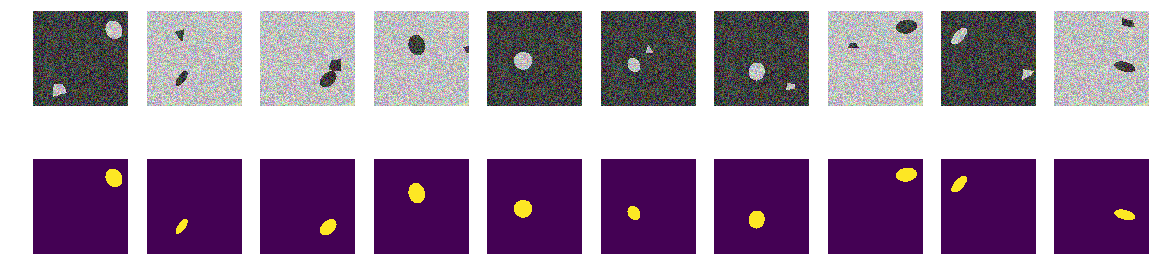
Now the same ellipses on the same sea, but the color of the sea and, accordingly, the ship is chosen randomly. If the sea is darker, the ship will be lighter and vice versa. Those. According to the brightness of the group of points, it is impossible to determine whether they are located outside the ellipse, i.e., the sea or it is the points inside the ellipse. And again we check our hypothesis that the network will find ellipses regardless of color.
defnext_pair():
    p = np.random.sample() - 0.5# это выбор цвета фон/эллипс
    r = np.random.sample()*(w_size-2*radius_max) + radius_max
    c = np.random.sample()*(w_size-2*radius_max) + radius_max
    r_radius = np.random.sample()*(radius_max-radius_min) + radius_min
    c_radius = np.random.sample()*(radius_max-radius_min) + radius_min
    rot = np.random.sample()*360
    rr, cc = ellipse(
      r, c,
      r_radius, c_radius,
      rotation=np.deg2rad(rot),
      shape=img_l.shape
    )
    if p > 0: #  если выбрали фон потемнее
        img = img_l.copy()
        img[rr, cc] = img_h[rr, cc]
    else: #  если выбрали фон светлее
        img = img_h.copy()
        img[rr, cc] = img_l[rr, cc]
    msk = np.zeros((w_size, w_size, 1), dtype='float32')
    msk[rr, cc] = 1.return img, msk
Now it is impossible to determine the background or ellipse by pixel and its surroundings. We also generate images and masks and look at the first 10 on the screen.
build picture masks
for k in range(train_num):
    img, msk = next_pair()
    train_x[k] = img
    train_y[k] = msk
fig, axes = plt.subplots(2, 10, figsize=(20, 5))
for k in range(10):
    axes[0,k].set_axis_off()
    axes[0,k].imshow(train_x[k])
    axes[1,k].set_axis_off()
    axes[1,k].imshow(train_y[k].squeeze())
input_layer = Input((w_size, w_size, 3))
output_layer = build_model(input_layer, 16)
model = Model(input_layer, output_layer)
model.compile(loss=bce_dice_loss, optimizer=Adam(lr=1e-3), metrics=[my_iou_metric])
model.load_weights('./keras.weights', by_name=False)
whileTrue:
    history = model.fit(train_x, train_y,
                        batch_size=32,
                        epochs=1,
                        verbose=1,
                        validation_split=0.1
                       )
    if history.history['my_iou_metric'][0] > 0.75:
        break
Train on 7372 samples, validate on 820 samples
Epoch 1/1
7372/7372 [==============================] - 56s 8ms/step - loss: 0.4652 - my_iou_metric: 0.5071 - val_loss: 0.0439 - val_my_iou_metric: 0.9005
Train on 7372 samples, validate on 820 samples
Epoch 1/1
7372/7372 [==============================] - 55s 7ms/step - loss: 0.1418 - my_iou_metric: 0.8378 - val_loss: 0.0377 - val_my_iou_metric: 0.9206The network easily copes and finds all ellipses. But even here there is a flaw in the implementation, and everything is obvious - the smaller of the two areas in the picture is the ellipse, another background. Perhaps this is an incorrect hypothesis, but still correct, add another polygon on the image of the same color as the ellipse.
Third option
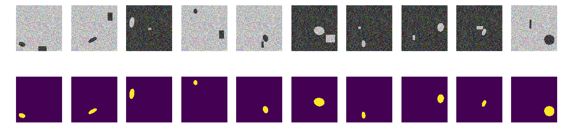
On each picture, we randomly select the color of the sea from two options and add an ellipse and a rectangle both different from the color of the sea. It turns out the same "sea", just painted "ship", but in the same picture add a rectangle of the same color as the "ship" and also with a randomly selected size. Now our assumption is more complicated, in the picture there are two equally colored objects, but we hypothesize that the network will still learn to choose the right object.
ellipse and rectangle drawing program
defnext_pair():#  выбираем также как и ранее параметры эллипса
    p = np.random.sample() - 0.5
    r = np.random.sample()*(w_size-2*radius_max) + radius_max
    c = np.random.sample()*(w_size-2*radius_max) + radius_max
    r_radius = np.random.sample()*(radius_max-radius_min) + radius_min
    c_radius = np.random.sample()*(radius_max-radius_min) + radius_min
    rot = np.random.sample()*360
    rr, cc = ellipse(
      r, c,
      r_radius, c_radius,
      rotation=np.deg2rad(rot),
      shape=img_l.shape
    )
    p1 = np.rint(np.random.sample()*(w_size-2*radius_max) + radius_max)
    p2 = np.rint(np.random.sample()*(w_size-2*radius_max) + radius_max)
    p3 = np.rint(np.random.sample()*(2*radius_max - radius_min) + radius_min)
    p4 = np.rint(np.random.sample()*(2*radius_max - radius_min) + radius_min)
  #  выбираем параметры прямоугольника/помехи, задаем четыре угла
    poly = np.array((
        (p1, p2),
        (p1, p2+p4),
        (p1+p3, p2+p4),
        (p1+p3, p2),
        (p1, p2),
    ))
    rr_p, cc_p = polygon(poly[:, 0], poly[:, 1], img_l.shape)
    in_sc = list(set(rr) & set(rr_p)) #  следим за тем, что бы прямоугольник#  не пересекался с эллипсом#  и сдвигаем его в сторону при необходимостиif len(in_sc) > 0:
        if np.mean(rr_p) > np.mean(in_sc):
            poly += np.max(in_sc) - np.min(in_sc)
        else:
            poly -= np.max(in_sc) - np.min(in_sc)
    rr_p, cc_p = polygon(poly[:, 0], poly[:, 1], img_l.shape)
    if p > 0:
        img = img_l.copy()
        img[rr, cc] = img_h[rr, cc]
        img[rr_p, cc_p] = img_h[rr_p, cc_p]
    else:
        img = img_h.copy()
        img[rr, cc] = img_l[rr, cc]
        img[rr_p, cc_p] = img_l[rr_p, cc_p]
    msk = np.zeros((w_size, w_size, 1), dtype='float32')
    msk[rr, cc] = 1.return img, msk
Just as before, we calculate pictures and masks and look at the first 10 pairs.
build picture masks ellipses and rectangles
for k in range(train_num):
    img, msk = next_pair()
    train_x[k] = img
    train_y[k] = msk
fig, axes = plt.subplots(2, 10, figsize=(20, 5))
for k in range(10):
    axes[0,k].set_axis_off()
    axes[0,k].imshow(train_x[k])
    axes[1,k].set_axis_off()
    axes[1,k].imshow(train_y[k].squeeze())
input_layer = Input((w_size, w_size, 3))
output_layer = build_model(input_layer, 16)
model = Model(input_layer, output_layer)
model.compile(loss=bce_dice_loss, optimizer=Adam(lr=1e-3), metrics=[my_iou_metric])
model.load_weights('./keras.weights', by_name=False)
whileTrue:
    history = model.fit(train_x, train_y,
                        batch_size=32,
                        epochs=1,
                        verbose=1,
                        validation_split=0.1
                       )
    if history.history['my_iou_metric'][0] > 0.75:
        break
Train on 7372 samples, validate on 820 samples
Epoch 1/1
7372/7372 [==============================] - 57s 8ms/step - loss: 0.7557 - my_iou_metric: 0.0937 - val_loss: 0.2510 - val_my_iou_metric: 0.4580
Train on 7372 samples, validate on 820 samples
Epoch 1/1
7372/7372 [==============================] - 55s 7ms/step - loss: 0.0719 - my_iou_metric: 0.8507 - val_loss: 0.0183 - val_my_iou_metric: 0.9812It was not possible to confuse the network with rectangles and our hypothesis is confirmed. At the Airbus competition, everyone, judging by examples and discussions, was a single vessel, and several vessels were quite close by. Ellipse from the rectangle - i.e. the ship is different from the house on the shore, the network is different, although the polygons are of the same color as the ellipses. The point is not in color, because both the ellipse and the rectangle are equally randomly colored.
Fourth option
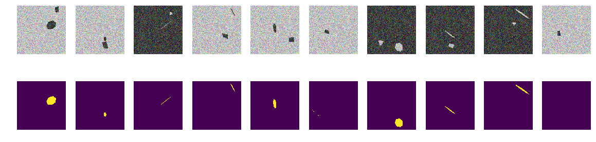
Perhaps the network is distinguished by rectangles - correct, distort them. Those. the network easily finds both closed areas regardless of shape and discards the one that is rectangle. This is the author's hypothesis - let's check it, for which we will add not rectangles, but quadrilateral polygons of arbitrary shape. And again our hypothesis is that the network will distinguish an ellipse from an arbitrary quadrilateral polygon of the same coloring.
You can certainly get into the inside of the network and look at the layers there and analyze the meaning of weights and shifts. The author is interested in the resulting behavior of the network, the judgment will be based on the result of the work, although it is always interesting to look inside.
make changes to the generation of images
defnext_pair():
    p = np.random.sample() - 0.5
    r = np.random.sample()*(w_size-2*radius_max) + radius_max
    c = np.random.sample()*(w_size-2*radius_max) + radius_max
    r_radius = np.random.sample()*(radius_max-radius_min) + radius_min
    c_radius = np.random.sample()*(radius_max-radius_min) + radius_min
    rot = np.random.sample()*360
    rr, cc = ellipse(
      r, c,
      r_radius, c_radius,
      rotation=np.deg2rad(rot),
      shape=img_l.shape
    )
    p0 = np.rint(np.random.sample()*(radius_max-radius_min) + radius_min)
    p1 = np.rint(np.random.sample()*(w_size-radius_max))
    p2 = np.rint(np.random.sample()*(w_size-radius_max))
    p3 = np.rint(np.random.sample()*2.*radius_min - radius_min)
    p4 = np.rint(np.random.sample()*2.*radius_min - radius_min)
    p5 = np.rint(np.random.sample()*2.*radius_min - radius_min)
    p6 = np.rint(np.random.sample()*2.*radius_min - radius_min)
    p7 = np.rint(np.random.sample()*2.*radius_min - radius_min)
    p8 = np.rint(np.random.sample()*2.*radius_min - radius_min)
    poly = np.array((
        (p1, p2),
        (p1+p3, p2+p4+p0),
        (p1+p5+p0, p2+p6+p0),
        (p1+p7+p0, p2+p8),
        (p1, p2),
    ))
    rr_p, cc_p = polygon(poly[:, 0], poly[:, 1], img_l.shape)
    in_sc = list(set(rr) & set(rr_p))
    if len(in_sc) > 0:
        if np.mean(rr_p) > np.mean(in_sc):
            poly += np.max(in_sc) - np.min(in_sc)
        else:
            poly -= np.max(in_sc) - np.min(in_sc)
    rr_p, cc_p = polygon(poly[:, 0], poly[:, 1], img_l.shape)
    if p > 0:
        img = img_l.copy()
        img[rr, cc] = img_h[rr, cc]
        img[rr_p, cc_p] = img_h[rr_p, cc_p]
    else:
        img = img_h.copy()
        img[rr, cc] = img_l[rr, cc]
        img[rr_p, cc_p] = img_l[rr_p, cc_p]
    msk = np.zeros((w_size, w_size, 1), dtype='float32')
    msk[rr, cc] = 1.return img, msk
We calculate pictures and masks and look at the first 10 pairs.
we build pictures masks ellipses and polygons
for k in range(train_num):
    img, msk = next_pair()
    train_x[k] = img
    train_y[k] = msk
fig, axes = plt.subplots(2, 10, figsize=(20, 5))
for k in range(10):
    axes[0,k].set_axis_off()
    axes[0,k].imshow(train_x[k])
    axes[1,k].set_axis_off()
    axes[1,k].imshow(train_y[k].squeeze())
We start our network. Let me remind you that it is the same for all options.
input_layer = Input((w_size, w_size, 3))
output_layer = build_model(input_layer, 16)
model = Model(input_layer, output_layer)
model.compile(loss=bce_dice_loss, optimizer=Adam(lr=1e-3), metrics=[my_iou_metric])
model.load_weights('./keras.weights', by_name=False)
whileTrue:
    history = model.fit(train_x, train_y,
                        batch_size=32,
                        epochs=1,
                        verbose=1,
                        validation_split=0.1
                       )
    if history.history['my_iou_metric'][0] > 0.75:
        break
Train on 7372 samples, validate on 820 samples
Epoch 1/1
7372/7372 [==============================] - 56s 8ms/step - loss: 0.6815 - my_iou_metric: 0.2168 - val_loss: 0.2078 - val_my_iou_metric: 0.4983
Train on 7372 samples, validate on 820 samples
Epoch 1/1
7372/7372 [==============================] - 53s 7ms/step - loss: 0.1470 - my_iou_metric: 0.6396 - val_loss: 0.1046 - val_my_iou_metric: 0.7784
Train on 7372 samples, validate on 820 samples
Epoch 1/1
7372/7372 [==============================] - 53s 7ms/step - loss: 0.0642 - my_iou_metric: 0.8586 - val_loss: 0.0403 - val_my_iou_metric: 0.9354
The hypothesis is confirmed, polygons and ellipses are easily distinguishable. The attentive reader will note here - of course they are different, a nonsense question, any normal AI can distinguish a second-order curve from the first line. Those. the network easily determines the presence of a boundary in the form of a second order curve. We will not argue, replace the oval by the heptagon and check.
The fifth experiment, the most difficult
There are no curves, only flat faces of regular inclined and rotated heptagons and arbitrary quadrangular polygons. Let us change the image / mask generator to the change function - only the projections of regular hexagons and arbitrary quadrangular polygons of the same color.
final editing of the image generation function
defnext_pair(_n = 7):
    p = np.random.sample() - 0.5
    c_x = np.random.sample()*(w_size-2*radius_max) + radius_max
    c_y = np.random.sample()*(w_size-2*radius_max) + radius_max
    radius = np.random.sample()*(radius_max-radius_min) + radius_min
    d = np.random.sample()*0.5 + 1
    a_deg = np.random.sample()*360
    a_rad = np.deg2rad(a_deg)
    poly = [] #  строим точки семиугольникаfor k in range(_n):
        #  сначала точки правильного семиугольника#  с_х с_у -координаты центра
        poly.append(c_x+radius*math.sin(2.*k*math.pi/_n))
        poly.append(c_y+radius*math.cos(2.*k*math.pi/_n))
        #  сжимаем\проецируем семиугольник#  на произвольную от 0.5 до 1.5 величину
        poly[-2] = (poly[-2]-c_x)/d +c_x
        poly[-1] = (poly[-1]-c_y) +c_y
        #  поворачиваем на случайный угол
        poly[-2] = ((poly[-2]-c_x)*math.cos(a_rad)\
                        - (poly[-1]-c_y)*math.sin(a_rad)) + c_x
        poly[-1] = ((poly[-2]-c_x)*math.sin(a_rad)\
                        + (poly[-1]-c_y)*math.cos(a_rad)) + c_y
    poly = np.rint(poly).reshape(-1,2)
    rr, cc = polygon(poly[:, 0], poly[:, 1], img_l.shape)
    p0 = np.rint(np.random.sample()*(radius_max-radius_min) + radius_min)
    p1 = np.rint(np.random.sample()*(w_size-radius_max))
    p2 = np.rint(np.random.sample()*(w_size-radius_max))
    p3 = np.rint(np.random.sample()*2.*radius_min - radius_min)
    p4 = np.rint(np.random.sample()*2.*radius_min - radius_min)
    p5 = np.rint(np.random.sample()*2.*radius_min - radius_min)
    p6 = np.rint(np.random.sample()*2.*radius_min - radius_min)
    p7 = np.rint(np.random.sample()*2.*radius_min - radius_min)
    p8 = np.rint(np.random.sample()*2.*radius_min - radius_min)
    poly = np.array((
        (p1, p2),
        (p1+p3, p2+p4+p0),
        (p1+p5+p0, p2+p6+p0),
        (p1+p7+p0, p2+p8),
        (p1, p2),
    ))
    rr_p, cc_p = polygon(poly[:, 0], poly[:, 1], img_l.shape)
    in_sc = list(set(rr) & set(rr_p))
    if len(in_sc) > 0:
        if np.mean(rr_p) > np.mean(in_sc):
            poly += np.max(in_sc) - np.min(in_sc)
        else:
            poly -= np.max(in_sc) - np.min(in_sc)
    rr_p, cc_p = polygon(poly[:, 0], poly[:, 1], img_l.shape)
    if p > 0:
        img = img_l.copy()
        img[rr, cc] = img_h[rr, cc]
        img[rr_p, cc_p] = img_h[rr_p, cc_p]
    else:
        img = img_h.copy()
        img[rr, cc] = img_l[rr, cc]
        img[rr_p, cc_p] = img_l[rr_p, cc_p]
    msk = np.zeros((w_size, w_size, 1), dtype='float32')
    msk[rr, cc] = 1.return img, msk
Just as before we build arrays and look at the first 10.
build picture masks
for k in range(train_num):
    img, msk = next_pair()
    train_x[k] = img
    train_y[k] = msk
fig, axes = plt.subplots(2, 10, figsize=(20, 5))
for k in range(10):
    axes[0,k].set_axis_off()
    axes[0,k].imshow(train_x[k])
    axes[1,k].set_axis_off()
    axes[1,k].imshow(train_y[k].squeeze())
input_layer = Input((w_size, w_size, 3))
output_layer = build_model(input_layer, 16)
model = Model(input_layer, output_layer)
model.compile(loss=dice_loss, optimizer=Adam(lr=1e-3), metrics=[my_iou_metric])
model.load_weights('./keras.weights', by_name=False)
whileTrue:
    history = model.fit(train_x, train_y,
                        batch_size=32,
                        epochs=1,
                        verbose=1,
                        validation_split=0.1
                       )
    if history.history['my_iou_metric'][0] > 0.75:
        break
Train on 7372 samples, validate on 820 samples
Epoch 1/1
7372/7372 [==============================] - 54s 7ms/step - loss: 0.5005 - my_iou_metric: 0.1296 - val_loss: 0.1692 - val_my_iou_metric: 0.3722
Train on 7372 samples, validate on 820 samples
Epoch 1/1
7372/7372 [==============================] - 52s 7ms/step - loss: 0.1287 - my_iou_metric: 0.4522 - val_loss: 0.0449 - val_my_iou_metric: 0.6833
Train on 7372 samples, validate on 820 samples
Epoch 1/1
7372/7372 [==============================] - 52s 7ms/step - loss: 0.0759 - my_iou_metric: 0.5985 - val_loss: 0.0397 - val_my_iou_metric: 0.7215
Train on 7372 samples, validate on 820 samples
Epoch 1/1
7372/7372 [==============================] - 52s 7ms/step - loss: 0.0455 - my_iou_metric: 0.6936 - val_loss: 0.0297 - val_my_iou_metric: 0.7304
Train on 7372 samples, validate on 820 samples
Epoch 1/1
7372/7372 [==============================] - 52s 7ms/step - loss: 0.0432 - my_iou_metric: 0.7053 - val_loss: 0.0215 - val_my_iou_metric: 0.7846
Train on 7372 samples, validate on 820 samples
Epoch 1/1
7372/7372 [==============================] - 53s 7ms/step - loss: 0.0327 - my_iou_metric: 0.7417 - val_loss: 0.0171 - val_my_iou_metric: 0.7970
Train on 7372 samples, validate on 820 samples
Epoch 1/1
7372/7372 [==============================] - 52s 7ms/step - loss: 0.0265 - my_iou_metric: 0.7679 - val_loss: 0.0138 - val_my_iou_metric: 0.8280Results
As we can see, the network distinguishes the projections of regular heptagons and arbitrary quadrilateral polygons with an accuracy of 0.828 on the test set. Network training is stopped at an arbitrary value of 0.75 and most likely the accuracy should be much better. If we proceed from the thesis that the network finds primitives and their combinations define an object, then in our case there are two areas with their average differing from the background, there are no primitives in the understanding of man. There are no clear, monochromatic lines, and corners, respectively, not, only areas with very similar boundaries. Even if lines are drawn, then both objects in the picture are built from identical primitives.
A question for connoisseurs - what does the network consider to be a sign that distinguishes "ships" from "interference"? Obviously, this is not the color or shape of the borders of the ships. You can of course continue to continue the study of this abstract construction "sea" / "ships", we are not an Academy of Sciences and can conduct research solely out of curiosity. We can change heptagons to octagons or fill in a picture with regular five and six squares and see if the network will distinguish them or not. I leave it for the readers - although it also became interesting to me whether the network can count the number of corners of a polygon and, for a test, place in the picture not regular polygons, but their random projections.
There are other, no less interesting properties of such ships, and such experiments are useful in that we set all the probabilistic characteristics of the set under study and the unexpected behavior of well-studied networks will add knowledge and benefit.
The background is random, the color is random, the place of the ship / ellipse is random. There are no lines in the pictures, there are areas with different characteristics, but there are no monochrome lines! In this case, of course there are simplifications and the task can be complicated - for example, choosing colors like 0.0 ... 0.9 and 0.1 ... 1.0 - but there is no difference for the network. The network can and does find patterns that differ from those that a person clearly sees and finds.
If someone from the readers is interested, you can continue to research and tinkering in the networks, if something does not work or is not clear, or suddenly a new and good idea appears and amazes with its beauty, then you can always share with us or ask the masters (and grandmasters too) and ask for qualified help in the ODS community.