September 5, 2016 at 18:58
Voronoi diagram and its application
Good all the time of the day, dear visitors of the site Habrahabr. In this article, I would like to tell you about what a Voronoi diagram is (shown in the picture below), about various algorithms for constructing it (for  ,
,  - intersection of half-planes,
  - Fortune's algorithm) and some subtleties of implementation (in C ++).
Many interesting uses of the chart and some interesting facts about it will also be considered. It will be interesting!
Layout of the article:
- Necessary concepts and definitions
- Algorithms of construction
- Applications
- Interesting facts
- References
- Fortune's algorithm) and some subtleties of implementation (in C ++).
Many interesting uses of the chart and some interesting facts about it will also be considered. It will be interesting!
Layout of the article:
- Necessary concepts and definitions
- Algorithms of construction
- Applications
- Interesting facts
- References
It is worth noting that in this article only algorithms for constructing a Voronoi diagram on a plane will be considered. Along the way, we will consider some other algorithms necessary for constructing a diagram — an algorithm for determining the point of intersection of two segments, an O'Rourke algorithm for the intersection of two convex polygons, and an algorithm for constructing a “coastline”.
I must say right away that everything that will happen next is on the plane .
Well, before starting to understand what this is - a Voronoi diagram, I’ll remind you of some concepts of the geometric objects we need (it is assumed, however, that you are already familiar with the definitions of a point, line, ray, line segment, polygon, vertex and edge of a polygon, vector and the intuitive concept of splitting a plane):
A simple polygon is a polygon without self-intersections. We will consider only simple polygons.
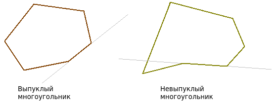
Non-convex polygon- this is a polygon in which there are two vertices such that a line is drawn through them that intersects the given polygon elsewhere, except for the edge connecting these vertices (see the picture).
A convex polygon is a polygon at which the extensions of the sides do not intersect others its sides (see picture). Other definitions are available on Wikipedia .
It is from convex polygons that the diagram will consist. Why precisely from convex? Because they are nothing more than the intersection of half-planes (as we will see later), which are convex figures, and here is why the intersection of convex figures is a convex figure, I suggest you find out for yourself (there is a proof, for example, in the book [2] ).
Since I started talking about half-planes, I can smoothly move on to the diagram itself — it consists of the so-called loci — regions in which there are all points that are closer to a given point than to all the others. In the Voronoi diagram, loci are convex polygons.
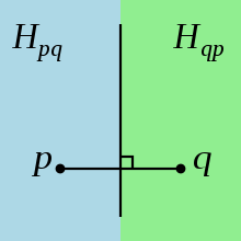
How to build a locus? By definition, it will be constructed as follows: let a set of n points be given, for which we are constructing a diagram. Take a specific point p , for which we construct a locus, and another point from the set given to us - q (not equal to p ). Draw a line connecting these two points, and draw a line, which will be the middle perpendicular of this segment. This straight line divides the plane into two half-planes - in one lies the point p , in the other lies the point q . In this case, the loci of these two points are the resulting half-planes. That is, in order to construct the locus of the point p , it is necessary to obtain the intersection of all such half-planes (i.e., in place of qall points of this set except p ) will be visited .
The point for which the locus is built is called the site . In the following picture, loci are marked in different colors.

Algorithms for constructing a diagram are precisely none other than algorithms for constructing these same loci for all points from a given set. Loci in this problem are also called Voronoi polygons or Voronoi cells .
Finally, we formulate the definition of the Voronoi diagram of n points on the plane (n is a positive integer) - this is a partition of the plane consisting of n loci (for each point at the locus). Again, another definition can be found on Wikipedia .
By the way, here is a site with an interactive color visualizer of the Voronoi diagram, you can click on the areayourself and sticksee how the chart is built.
If you are interested in how the diagram appeared and why it bears the name of Voronoi, then you should take a look under the spoiler below.
We will learn how to build a Voronoi diagram. We will consider 4 algorithms, 2 of which are detailed (1 with implementation, a full implementation of the Fortune algorithm will be discussed in a separate article), 2 more briefly (and without implementation):
After some algorithms are described, its implementation in C ++ will be given. For implementation, we used the SplashGeom © library that we wrote - a link to github , which has everything you need to implement many algorithms of computational geometry on the plane and some in space. I ask you not to judge strictly this library, it is still in the stage of active development and improvement, however, all comments will be heard.
If you are interested in other implementations, here are some more:
Now let's move on to a direct examination of the algorithms:
Algorithm for plotting the Voronoi diagram “forehead” for
The idea here is not to intersect the half-planes, but the middle perpendiculars of the segments (because it’s simpler, you must agree) connecting this point with all other points. That is, we, following the definition of the Voronoi cell, will construct a locus for the point p like this:
The algorithm can also be found on e-maxx.ru .
If you wish, you can independently implement this algorithm using SplashGeom ©. In this article, its implementation is not given, because this algorithm in practice is much inferior to at least the following ...
Algorithm for constructing a Voronoi diagram by intersecting half-planes beyond
This algorithm can already be used in practice, since it does not have such great computational complexity. For him, we need: to be able to intersect segments and lines, to be able to intersect convex polygons, to be able to intersect half-planes, and to be able to combine the resulting loci into a diagram.
The main catch here, I believe, is to implement the normal intersection of convex polygons, because there are unpleasant degenerate cases (the vertices and / or sides of the polygons coincide; if the polygon intersects itself, you need to think carefully to adapt the O'Rourke algorithm for correct operation in in this case).
I must say right away that we are restricting the entire scope of actions to a bounding rectangle - the half-planes will cut off the parts from it that we will intersect with each other. This solves the problem of infinite cells in the diagram.
And we need precisely the intersection points, and not just the determination of its presence. In SplashGeom © this is - for example, the implementation of the intersection of lines and segments:
Now we realize the intersection of the polygons. You can, of course, do this for , where n and m are the number of vertices of the first and second polygon, respectively - intersect each side of the first polygon with each side of the second, writing the intersection points, and also check the points of belonging to another polygon, but we, in order to achieve the best speed, we will cross according to the O'Rourke algorithm (the original description of the algorithm is [3] ).
Also, one of the options for its description can be found on algolist.ru . Our implementation is based on the description of the algorithm in the book [1] (p. 334), with some complementary ideas. I note right away that this implementation does not take into account cases when polygonsthere are common sides (as noted in the book [1] , this case requires a separate consideration), however, cases with common vertices work correctly.
Under the spoiler below you can see a general description of the algorithm.
Well, in SplashGeom © it looks like this:
I hope this description and code will be useful to you.
So, we have everything you need to build the intersection of half-planes. Well, let's do it, and let's do it not just, but in a clever way - due to the associativity of the operation of intersecting half-planes, we can intersect them in any order, which means we will intersect two planes, then intersect two more, and then intersect their intersections, this is already faster than crossing everything separately.
So it’s advisable to use recursion(the mood immediately went bad) - its work here is quite understandable, see for yourself:
Now we have the Voronoi polygon of a given point, it's time to add it to the diagram. There are no particular problems with this, because we get regions in an arbitrary order, and they are not related to each other (unlike the implementation in the Fortune algorithm, where you can go to a neighboring locus by a pointer to an edge):
So, we learned how to build a Voronoi diagram for, it has the form of a vector (list) of loci. The disadvantage of this solution is that information about neighbors cannot be obtained (perhaps this disadvantage can be eliminated by an improved implementation).
Much more information can be obtained from the RSDS ( DCEL ). This structure will be used in Fortune's algorithm.
Next, the Fortune algorithm will be described using a sweeping straight line and “coastline”(prepare swimwear and swimming trunks - go to the beach) . In my opinion, this is the most acceptable option if you want to implement the construction of the Voronoi diagram and build it with the "speed" of light .
Fortune's algorithm for constructing the Voronoi diagram for
In 1987, Steve Fortune proposed an algorithm for plotting a chart beyond. Of course, it is not the only construction algorithm with such asymptotics, but it is quite understandable and not very difficult to implement (and, moreover, very beautiful and mathematical! ), So I chose it.
Fortune algorithm materials can be found here , here , here and here .
By the way, an article on Habrahabr has already been devoted to the consideration of this algorithm .
So, the main idea of the algorithm is the so-called sweep line. It is used in many algorithms of computational geometry, because it allows you to conveniently simulate the motion of a straight line along a certain set of objects (for example, a sweep line is also used in the algorithm for intersecting n segments).
Before we start talking about how and what we will do, let's see how the sweep line moves (taken from here ):
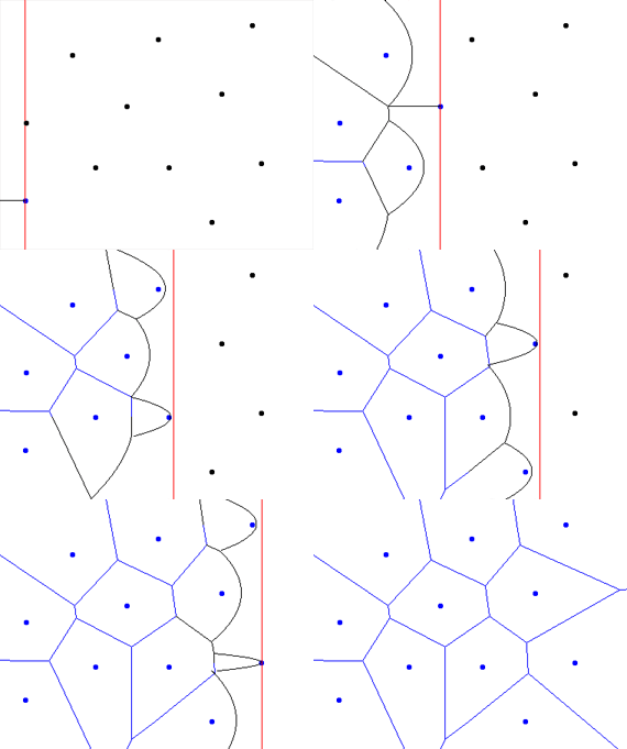
Nice, isn't it? In the implementation, everything is approximately the same, only the RFP usually moves from top to bottom, and not from left to right, and in fact, everything is not so smooth, but comes from event to event (see below), that is, discrete .
There are n sites (points on the plane). There is a sweeping line that moves (for example) “from top to bottom,” that is, from the site with the largest ordinate to the site with the smaller (from event to event, to be precise). It should be noted right away that only sites that are higher or on a sweeping line have an impact on charting .
When the ZP gets to the next site (a point event) , a new parabola (arch) is created, the focus of this site is, and the director is a sweeping line ( about the parabola on Wikipedia) This parabola divides the plane into two parts - the “inner” area of the parabola corresponds to the points that are closer to the site, and the “outer” area corresponds to the points that are closer to the sweep line, but the points lying on the parabola are equidistant from the site and the GP. The parabola will change depending on the position of the RFP to the site - the further the RFP goes down from the site, the more the parabola expands, however at the very beginning it is generally a segment (“directed” upwards).
Then the parabola expands, it has two break points- points of its intersection with other parabolas (“coastline”). In the “coastline” we store parabolic arcs from one point of their intersection with each other to the other, and so the beach line turns out. In fact, in this algorithm we simulate the movement of this “coastline”. because these same break points move exactly along the edges of the Voronoi cells (after all, it turns out that the control points are equidistant from both sites to which these parabolas correspond, and even from the GP).
And just at that moment when two control points - on one of the different parabolas - “meet”, that is, as if turn into one, this point becomes the top of the Voronoi cell (circle event occurs )), and at that time the arc that was between these two points - “collapses” and is removed from the “coastline”. Next, we simply connect this point with the previous corresponding one and get the edge of the Voronoi cell.
So, when sweep line moves down, we encounter two types of events :
The event of a point is the hit of a PO on one of the sites, so we create a new parabola corresponding to this site, and two break points are added (in fact, at first it’s one, but when expanding the arch there are already two) —the intersection points of parabolas with a coastline (that is, with the front of existing parabolas). It should be noted that in this algorithm the parabola (or rather its part belonging to the “coastline” - the arch ) is “inserted into the coastline” only in case of a point event, that is, a new arch can appear only when processing a point event .
By the way, the following pictures show why the associations of such “pieces of parabolas” are called the “coastline”.
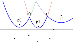

The circle event is the appearance of a new vertex of the Voronoi cell along with the removal of one arch, because the appearance of a new vertex of the diagram here means that there were three arches, the left, middle and right, the middle “collapses” due to the approach of the left and right points of the arches and a new vertex is obtained Voronoi diagrams. It is worth noting that in this algorithm a parabola (arch) is removed from the “coastline” only in the event of a circle event, that is, an arch can be deleted only when processing a circle event .
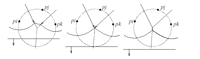
There is a theorem which says that the vertex of the Voronoi diagram always lies at the intersection of exactly three edges of the diagram, and there is a consequence of this theorem, which states that the vertex of the diagram is the center of a circle passing through three sites and the distance from this point to the sweeping line is also equal to the radius of this circle (this is a property of points lying on the “coastline”). This is the key point , because it is when the lowest point of the circle passing through the three sites lies below or on the sweeping line that we push the circle event with this lowest point into the event queue, because when the line hits it, we get the top Voronoi diagrams.
Importantthat with any event (point or circle) one particular arch is connected, and vice versa. This is useful when handling events. We also must not forget that you need time to add ribs in RSBC ( DCEL ) (item 1 in the structures, see. Below), so you need to understand the relationship with the arch ribs.
Thus, the movement of the direct discrete - direct at any time either on site , or at the bottom point of the circle passing through the three sites, the center of which - new vertex Voronoi diagram. Perfectly.
General algorithm :
The implementation of the Fortune algorithm will be considered in detail in a separate article , however, here are some developments that may help in understanding it.
To implement this algorithm, we need several structures (classes), namely:
Having such data structures, we can write an implementation of the general algorithm:
All the logic and complexity in HandlePointEvent () and HandleCircleEvent () will be the subject of a separate article, hereinafter I will give some auxiliary functions that will later help in implementation.
We need to be able to get the intersection of two parabolas (arches) depending on the position of the RFP. The equation of a parabola with focus at the point x 'and y' and the director, whose position along the y axis is l, is given by the following equation (it can be derived): By the way, the fraction in front of the bracket is the focal parameter of this parabola. From here we can “pull out” the corresponding coefficients of the parabola equation and solve the system of two nonlinear equations in a simple way - we subtract one from the other, and then substitute the found roots in the first, we get two points. We are interested in the point that is lower (that is, with a smaller ordinate), because the highest point lies behind the “coastline”. The described actions are reflected in the following code:

When processing a circle event, we will need to determine the center and the lowest point of the circle constructed from the foci of the three arches (sites). There are some analytical algorithms for constructing a circle using three points (by construction we mean getting its center and radius), in our program this is done ( thanks to the algolist ) - we connect the first two points and the second two points by segments. The center lies at the intersection of the middle perpendiculars, the radius is the distance from the center to any of the three points. Fast and beautiful:
A point event is when we pulled a PointEvent out of the queue. What is in it? It has only the site with which this event is associated.
What do we do when processing it? We add a new arch to the “coastline”, setting up all the connections “as needed” in the tree, and check if the circle event has appeared in one of three possible cases - we need to check all cases in which the new site can participate.
What do we do when adding an arch? We look for a place for it in our binary “coastline” tree (at the x coordinate), then insert it.
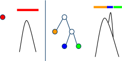
What do we do when pasted? We found a pointer to the arch with which the new intersects at two points (the case when the intersection point hits exactly one of the control points is considered separately - there will be an intersection with two parabolas - left and right).
That is, we take this arch, which “breaks”, and instead we insert as many as 5 nodes (there was 1, it became 5, yes) - arch1, bp1, arch2, bp2, arch3. Arch1 is the left part of the arch that the new intersects, that is, it is the piece to the left of the left break point, bp1 is the left break point (the left intersection of the new arch), arch2 is the new arch in person, bp2 is the right break point (right intersection of the new arch), arch3 is the right piece of the arch that the new intersects.
It is worth noting that the point event gives rise to a new edge (or edges, there are cases) of the Voronoi diagram.
One of the possible options for adding a new arch to the “coastline” is presented in this article on Habré , our version is described above, and is more similar to the one proposed here .
A circle event is when we pulled out a CircleEvent from the queue.
What is in it? There is a point in it - this is the lowest point of a certain circle that passes through three sites, and an arch that should be removed. There are two control points in the tree, and she herself, the control points will eventually turn into one, and the arch must be carefully removed from the tree, rebuilding all the “parent-child relationships”. In fact, processing this event replaces three nodes in the tree with one (two break points and an arch with one break point).
It is worth noting that the circle event completes two edges of the Voronoi diagram, that is, when this event is processed, the edges will end.
I’ll also say that an important part of event processing is how we monitor the growth of edges, add them to the list and complete the edges, that is, so that in the end they are all “finished” and either be finite or rest against the bounding rectangle.
Since we will already receive RSDS ( DCEL ) at the output , we can get enough information - for each edge we know the corresponding site, we can get the "twin" of this edge, find out the site for it and voila - we recognized the neighbor (so, going around to the list, we can create lists of neighbors for all sites, and this is already an achievement, since everything happened in the end for+  = ).
= ).
Moreover, if the edge has a “zero” site, then we are on the “boundary site” - a site with an “infinite” locus. Hmm, but this will allow us to build a convex hull of the initial set of points;in the end, great.
Well, in general, RSDS is essentially a graph, so you can continue to work with this list in many graph algorithms.
The recursive algorithm for constructing the Voronoi diagram for
This algorithm is given in the book [1] (p. 260), here I will only give the construction algorithm itself, since we did not implement this option, although it is a good analogy to the Fortune algorithm.
The general description of the algorithm is not complicated, but the algorithm has its own subtleties, which you can find in the specified book.
An exhaustive list of all applications of the Voronoi diagram can be found here . I’ll mention some of them that seemed to me the most interesting (many information was taken from [1] ):
In computational geometry, the Voronoi diagram is needed primarily for solving the problem of proximity of points, or rather, the diagram gives a special gain in solving the problem of ALL closest neighbors(not those that turn on music loudly, but though ..) , because similar methods are not so simple ( [1] ). Using the Voronoi diagram, one can construct a convex hull behind (look at the “ray” edges, find the sites to which they belong, and include them in the hull).
There is also an important connection between the Voronoi diagram and the Delaunay triangulation , which allows one to build one after another, because they are dual to each other (we connect adjacent sites by edges, as a result we get Delaunay triangulation - Wikipedia ).
An example of using the Voronoi diagram in game dev can be found, for example, in this article - here the navigation system in the game engine is based on the diagram.
It is possible, and even likely, that various geolocation software uses Voronoi diagrams. Geolocation reference systems can use the Voronoi diagram to determine, for example, the nearest grocery store, for various search and analysis of the location.
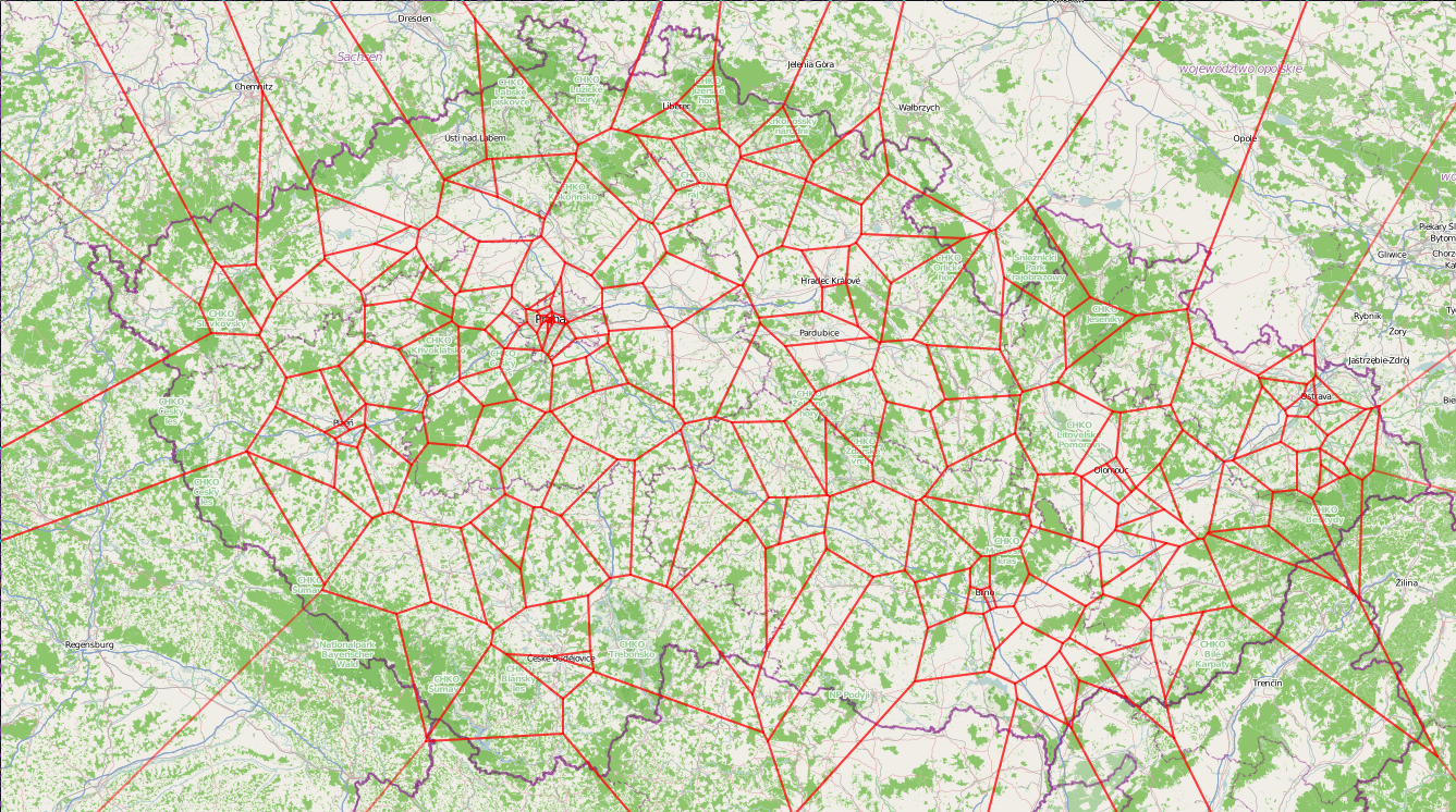
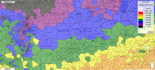
Here you can also mention the use of the chart in cartography - to outline the boundaries of the regions and further analysis based on them. Anyway, any geographic diagrams showing the distribution of something can be clearly illustrated using the colored Voronoi diagrams, and there we will see the transition of the indicator we need (for example, temperature):
Well, of course, you can make various filter-photo handlers using the Voronoi diagram, getting some kind of “mosaic”.

But this is only the beginning of its application.
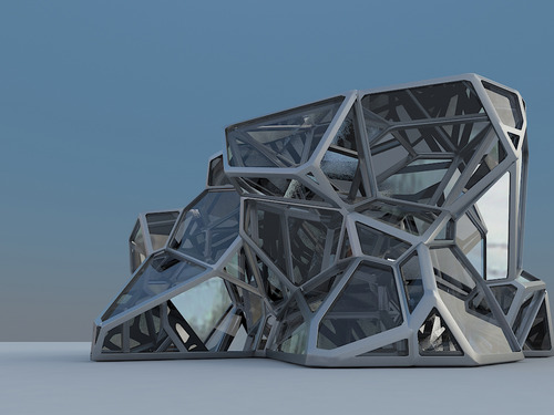
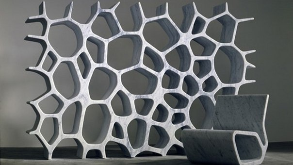
It is quite logical that people came up with the idea of using the Voronoi diagram in architecture and design, since it itself is a beautiful drawing, a kind of “geometric web”, so there are many cases of using it as one of the main elements of a composition or even a frame all creation. Examples:


From [1] :
This article does not discuss Voronoi’s 3D diagram, but it has many applications in physics and 3D modeling of objects. Various kinds of grids (and skeletons ) of objects in space can be constructed using the Voronoi diagram (however, more often using Delaunay triangulation ).
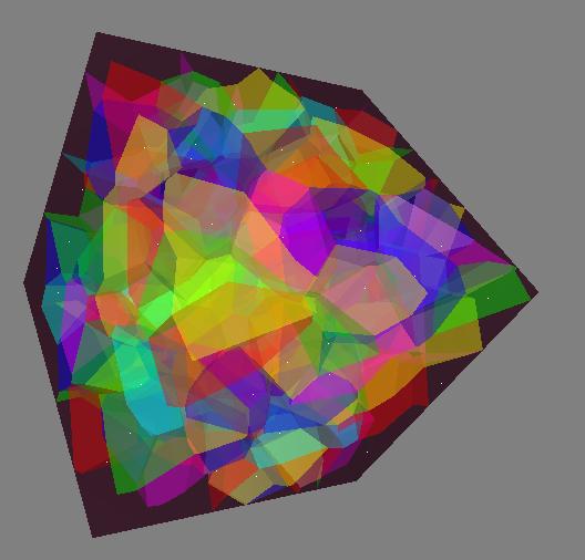

3D scanning (and computer vision ) of various objects can also use the Voronoi diagram and Delaunay triangulation, it is also closely related to robotics - the movement of the robot taking into account obstacles in the way.

From [1] :
Here is another interesting article about using the Voronoi diagram.
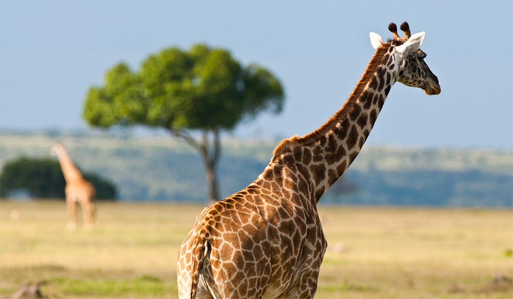
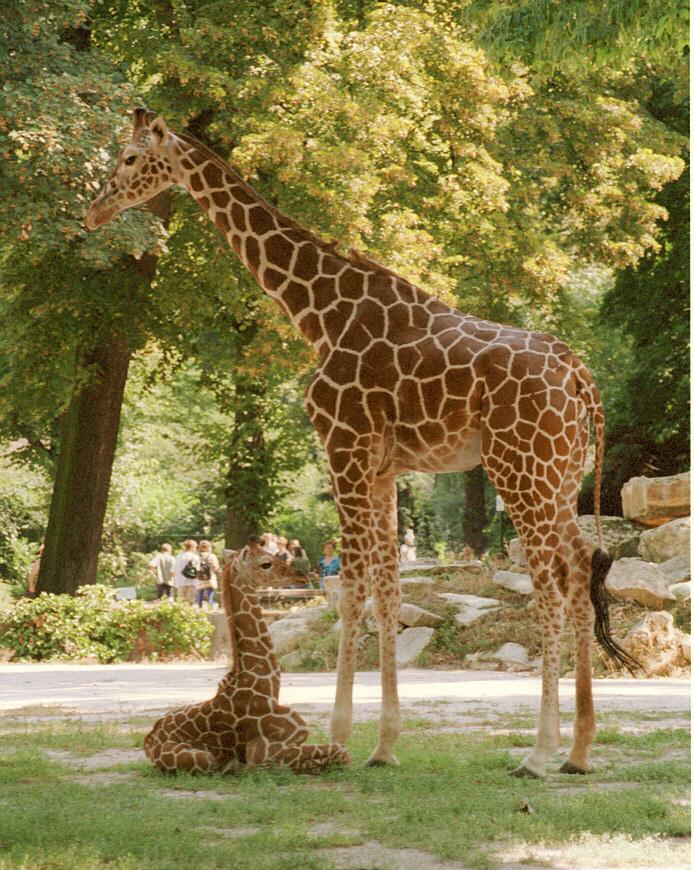
Nature is an amazing thing, because it turns out that the color of the giraffe actually looks like a Voronoi diagram. This is visible to the naked eye:
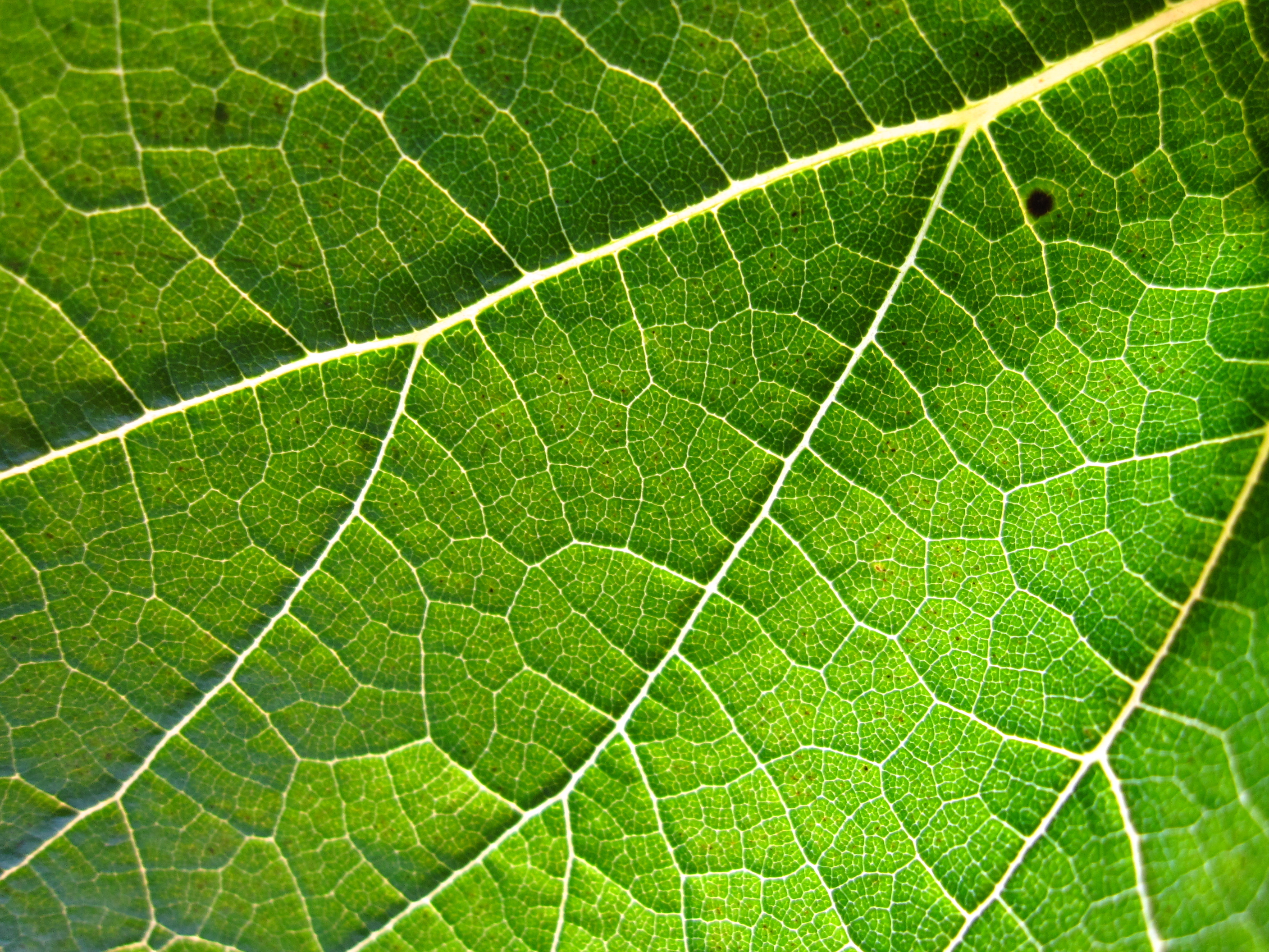
The following observation is also noteworthy, which shows that the diagram can be seen even on the leaves of trees:
By the way, a little less than a year ago, one incident was also associated with the Voronoi diagram - here it was used in the logo of the New Moscow project.

And - finally - a video in which you can see how the diagram appears with the growth of circles with centers in the sites:
Here we can draw an analogy with the spread of a fire that has several fire sources.
Well, our little trip to a world where everyone knows who is closest to them has come to an end. I hope you enjoyed this article and you really learned something new, useful and interesting.
Thanks for attention!
[1] Preparation F., Shaymos M. Computational geometry. Introduction (1989)
[2] Alexandrov A. D., Werner A. L., Ryzhik V. I. Stereometry. Geometry in space
[3] Joseph O'Rourke. Computational Geometry in C
»This article was prepared by Ilya Zakharkin, 1st year student of the Institute of Physics and Technology .
»First-year students of the FIVT MIPT Kirilenko Elena and Kasimova Nadezhda also helped in writing the library .
»In testing the library helped Yaroslav Spirin .
» Special thanks to the mentors Gadelshin Ilnur and Gafarov Rustam .
, - intersection of half-planes, - Fortune's algorithm) and some subtleties of implementation (in C ++).
Many interesting uses of the chart and some interesting facts about it will also be considered. It will be interesting!
Layout of the article:
- Necessary concepts and definitions
- Algorithms of construction
- Applications
- Interesting facts
- ReferencesIt is worth noting that in this article only algorithms for constructing a Voronoi diagram on a plane will be considered. Along the way, we will consider some other algorithms necessary for constructing a diagram — an algorithm for determining the point of intersection of two segments, an O'Rourke algorithm for the intersection of two convex polygons, and an algorithm for constructing a “coastline”.
Necessary concepts and definitions
I must say right away that everything that will happen next is on the plane .
Well, before starting to understand what this is - a Voronoi diagram, I’ll remind you of some concepts of the geometric objects we need (it is assumed, however, that you are already familiar with the definitions of a point, line, ray, line segment, polygon, vertex and edge of a polygon, vector and the intuitive concept of splitting a plane):
A simple polygon is a polygon without self-intersections. We will consider only simple polygons.
Non-convex polygon- this is a polygon in which there are two vertices such that a line is drawn through them that intersects the given polygon elsewhere, except for the edge connecting these vertices (see the picture).
A convex polygon is a polygon at which the extensions of the sides do not intersect others its sides (see picture). Other definitions are available on Wikipedia .
It is from convex polygons that the diagram will consist. Why precisely from convex? Because they are nothing more than the intersection of half-planes (as we will see later), which are convex figures, and here is why the intersection of convex figures is a convex figure, I suggest you find out for yourself (there is a proof, for example, in the book [2] ).
Since I started talking about half-planes, I can smoothly move on to the diagram itself — it consists of the so-called loci — regions in which there are all points that are closer to a given point than to all the others. In the Voronoi diagram, loci are convex polygons.
How to build a locus? By definition, it will be constructed as follows: let a set of n points be given, for which we are constructing a diagram. Take a specific point p , for which we construct a locus, and another point from the set given to us - q (not equal to p ). Draw a line connecting these two points, and draw a line, which will be the middle perpendicular of this segment. This straight line divides the plane into two half-planes - in one lies the point p , in the other lies the point q . In this case, the loci of these two points are the resulting half-planes. That is, in order to construct the locus of the point p , it is necessary to obtain the intersection of all such half-planes (i.e., in place of qall points of this set except p ) will be visited .
The point for which the locus is built is called the site . In the following picture, loci are marked in different colors.
Algorithms for constructing a diagram are precisely none other than algorithms for constructing these same loci for all points from a given set. Loci in this problem are also called Voronoi polygons or Voronoi cells .
Finally, we formulate the definition of the Voronoi diagram of n points on the plane (n is a positive integer) - this is a partition of the plane consisting of n loci (for each point at the locus). Again, another definition can be found on Wikipedia .
By the way, here is a site with an interactive color visualizer of the Voronoi diagram, you can click on the area
If you are interested in how the diagram appeared and why it bears the name of Voronoi, then you should take a look under the spoiler below.
Historical facts
(material taken from this site)
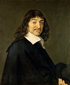
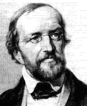
In general, the first use of this diagram is found in the work of Rene Descartes (1596-1650), "The Beginning of Philosophy" (1644). Descartes proposed dividing the universe into zones of gravitational influence of stars.

Only two centuries later, the famous German mathematician Johann Peter Gustav Lejeune-Dirichlet (1805 - 1859) introduced diagrams for two- and three-dimensional cases. Therefore, they are sometimes called Dirichlet diagrams.
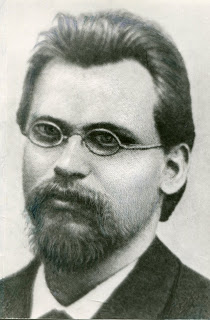
Well, already in 1908, the Russian mathematician Georgy Feodosievich Voronoi (April 16 (28), 1868 - November 7 (20), 1908) described this diagram for spaces of greater dimensions, since then the diagram bears his last name. Here is his brief biography (taken from Wikipedia ):
Georgy Feodosievich Voronoi was born in the village of Zhuravka, Poltava province (now Chernihiv region). Since 1889, he studied at St. Petersburg University with Andrei Markov . In 1894 he defended his master's thesis "On integers depending on the root of the equation of the third degree." In the same year he was elected professor at the University of Warsaw, where he studied chain fractions. Voronoi was trained by Vaclav Sierpinski . In 1897, Voronoi defended his doctoral dissertation "On a generalization of the algorithm for continued fractions", awarded the Bunyakovsky Prize.
A bit of history
(material taken from this site)
In general, the first use of this diagram is found in the work of Rene Descartes (1596-1650), "The Beginning of Philosophy" (1644). Descartes proposed dividing the universe into zones of gravitational influence of stars.
Only two centuries later, the famous German mathematician Johann Peter Gustav Lejeune-Dirichlet (1805 - 1859) introduced diagrams for two- and three-dimensional cases. Therefore, they are sometimes called Dirichlet diagrams.
Well, already in 1908, the Russian mathematician Georgy Feodosievich Voronoi (April 16 (28), 1868 - November 7 (20), 1908) described this diagram for spaces of greater dimensions, since then the diagram bears his last name. Here is his brief biography (taken from Wikipedia ):
Georgy Feodosievich Voronoi was born in the village of Zhuravka, Poltava province (now Chernihiv region). Since 1889, he studied at St. Petersburg University with Andrei Markov . In 1894 he defended his master's thesis "On integers depending on the root of the equation of the third degree." In the same year he was elected professor at the University of Warsaw, where he studied chain fractions. Voronoi was trained by Vaclav Sierpinski . In 1897, Voronoi defended his doctoral dissertation "On a generalization of the algorithm for continued fractions", awarded the Bunyakovsky Prize.
Construction Algorithms
We will learn how to build a Voronoi diagram. We will consider 4 algorithms, 2 of which are detailed (1 with implementation, a full implementation of the Fortune algorithm will be discussed in a separate article), 2 more briefly (and without implementation):
- Algorithm for plotting the Voronoi diagram “on the forehead”. Difficulty: ;
- Algorithm for constructing a Voronoi diagram by intersecting half-planes. Difficulty: ;
- Fortune's algorithm for constructing a Voronoi diagram on a plane. Difficulty: ;
- A recursive algorithm for constructing a Voronoi diagram. Difficulty: .
After some algorithms are described, its implementation in C ++ will be given. For implementation, we used the SplashGeom © library that we wrote - a link to github , which has everything you need to implement many algorithms of computational geometry on the plane and some in space. I ask you not to judge strictly this library, it is still in the stage of active development and improvement, however, all comments will be heard.
If you are interested in other implementations, here are some more:
- boost.polygon
- Steve Fortune website
- aewllin / openvoronoi
- Java implementation
- JavaScript implementation (there is also a visualizer)
Now let's move on to a direct examination of the algorithms:
Algorithm for plotting the Voronoi diagram “forehead” for
The idea here is not to intersect the half-planes, but the middle perpendiculars of the segments (because it’s simpler, you must agree) connecting this point with all other points. That is, we, following the definition of the Voronoi cell, will construct a locus for the point p like this:
- We get the n-1 straight line (middle perpendiculars), since we have drawn the middle perpendiculars of all the segments connecting this point p with the rest;
- We cross all the lines in pairs, we get the
 intersection points (because each line can intersect all the others, in the “worst case”);
 - We check all these points for the membership of each of the n-1 half-planes, that is, we already obtain the asymptotic behavior
 . Accordingly, those points that belong to all half-planes will be the vertices of the Voronoi cell of the point p ;
 - We perform the first three steps for all n points, we obtain the resulting asymptotics .
The algorithm can also be found on e-maxx.ru .
If you wish, you can independently implement this algorithm using SplashGeom ©. In this article, its implementation is not given, because this algorithm in practice is much inferior to at least the following ...
Algorithm for constructing a Voronoi diagram by intersecting half-planes beyond
This algorithm can already be used in practice, since it does not have such great computational complexity. For him, we need: to be able to intersect segments and lines, to be able to intersect convex polygons, to be able to intersect half-planes, and to be able to combine the resulting loci into a diagram.
Algorithm
- We get the n-1 straight line for the current site (as in the previous algorithm - the middle perpendiculars). These will be the “generators” of the half-planes;
- Now we have an n-1 half-plane. Each of these half-planes is given by a straight line from before. point and orientation, that is, which side of the line it is located. Orientation can be determined by the current site for which we are building a locus - it lies in the desired half-plane, and therefore its locus must lie in it;
- We cross all the half-planes - we can do it for - we get the locus for the current site;
- We perform the first three steps for all n points, we obtain the resulting asymptotics
 * = .
* = .
Implementation
The main catch here, I believe, is to implement the normal intersection of convex polygons, because there are unpleasant degenerate cases (the vertices and / or sides of the polygons coincide; if the polygon intersects itself, you need to think carefully to adapt the O'Rourke algorithm for correct operation in in this case).
I must say right away that we are restricting the entire scope of actions to a bounding rectangle - the half-planes will cut off the parts from it that we will intersect with each other. This solves the problem of infinite cells in the diagram.
The intersection of lines and segments
And we need precisely the intersection points, and not just the determination of its presence. In SplashGeom © this is - for example, the implementation of the intersection of lines and segments:
View code
// пересечение прямых
// kInfPoint - прямые параллельны, kNegInfPoint - прямые совпадают
Point2D Line2D::GetIntersection(const Line2D& second_line) const
{
	double cross_prod_norms = Vector2D(this->A, this->B).OrientedCCW(Vector2D(second_line.A, second_line.B));
	Point2D intersect_point;
	if (fabs(cross_prod_norms) <= EPS) /* A1 / A2 == B1 / B2 */ {
		if (fabs(this->B * second_line.C - second_line.B * this->C) <= EPS) /* .. == C1 / C2 */ {
			intersect_point = kNegInfPoint2D;
		} else {
			intersect_point = kInfPoint2D;
		}
	} else {
		double res_x = (second_line.C * this->B - this->C * second_line.B) / cross_prod_norms;
		double res_y = (second_line.A * this->C - this->A * second_line.C) / cross_prod_norms;
		intersect_point = Point2D(res_x, res_y);
	}
	return intersect_point;
}
// пересечение отрезков
Point2D Segment2D::GetIntersection(const Segment2D& second_seg) const
{
	Line2D first_line(*this);
	Line2D second_line(second_seg);
	Point2D intersect_point = first_line.GetIntersection(second_line);
	if (intersect_point == kNegInfPoint2D) {
		if (this->Contains(second_seg.b)) {
			intersect_point = second_seg.b;
		} else if (this->Contains(second_seg.a)) {
			intersect_point = second_seg.a;
		} else if (second_seg.Contains(this->b)) {
			intersect_point = this->b;
		} else if (second_seg.Contains(this->a)) {
			intersect_point = this->a;
		} else {
			intersect_point = kInfPoint2D;
		}
	} else if (!(this->Contains(intersect_point) && second_seg.Contains(intersect_point))) {
			intersect_point = kInfPoint2D;
	}
	return intersect_point;
}
Intersection of Convex Polygons
Now we realize the intersection of the polygons. You can, of course, do this for
, where n and m are the number of vertices of the first and second polygon, respectively - intersect each side of the first polygon with each side of the second, writing the intersection points, and also check the points of belonging to another polygon, but we, in order to achieve the best speed, we will cross according to the O'Rourke algorithm (the original description of the algorithm is [3] ). Also, one of the options for its description can be found on algolist.ru . Our implementation is based on the description of the algorithm in the book [1] (p. 334), with some complementary ideas. I note right away that this implementation does not take into account cases when polygonsthere are common sides (as noted in the book [1] , this case requires a separate consideration), however, cases with common vertices work correctly.
Under the spoiler below you can see a general description of the algorithm.
I want to know the O'Rourke algorithm!
Algorithm (for additional explanations, refer to the above sources):
The Motion function can be implemented in different ways, with us it returns the number (label) of the polygon whose edge we are moving. Conceptually, she does three things within herself:
- determines the case number - the current relative position of the edges of the first polygon and the edges of the second polygon. This is the main idea of the algorithm - viewing cases of the position of the edges relative to each other. All these four positions are well described in [1] ; in our implementation, the position is determined using the skew product of vectors on the plane;
- determines which edge of which polygon is now “inside”, that is, it lies “to the left” of the other edge, this is also checked with an oblique product (lies “to the left” if the endpoint lies “to the left”);
- Decides whether to write the current end of one of the edges to the intersection polygon. If this corresponds to the desired case and the rib inside, then you need to add, otherwise not.
- Until the maximum number of iterations has passed (it is proved that it is no more than 2 * (n + m)), we carry out the following instructions:
a). Take the current edges of the first and second polygons;
b) If they intersect - then we consider a point from the intersection: it may be that we just added it to the intersection polygon, then just ignore the addition, otherwise - if it is not the initial intersection point (that is, we have already made a circle), then add to intersection, otherwise we finish the algorithm - we met the intersection point, which was at the beginning;
in). Next (regardless of whether the current edges intersect or not), we call the Motion function, which is responsible for moving the window of the first (or second) polygon one edge forward, as well as for the possible addition of a vertex to the intersection polygon. The main actions take place precisely in the Movement . - If there were no intersection points, determine whether one polygon lies inside another (check whether the point belongs to a convex polygon behind O (log (number of vertices of the polygon)) - [1] , pp. 59-60). If it is, then return it, otherwise return an empty intersection.
The Motion function can be implemented in different ways, with us it returns the number (label) of the polygon whose edge we are moving. Conceptually, she does three things within herself:
- determines the case number - the current relative position of the edges of the first polygon and the edges of the second polygon. This is the main idea of the algorithm - viewing cases of the position of the edges relative to each other. All these four positions are well described in [1] ; in our implementation, the position is determined using the skew product of vectors on the plane;
- determines which edge of which polygon is now “inside”, that is, it lies “to the left” of the other edge, this is also checked with an oblique product (lies “to the left” if the endpoint lies “to the left”);
- Decides whether to write the current end of one of the edges to the intersection polygon. If this corresponds to the desired case and the rib inside, then you need to add, otherwise not.
Well, in SplashGeom © it looks like this:
Polygon Intersection Code
// для получения многоугольников, которые полуплоскости отсекают от ограничивающего прямоугольника
Convex2D Rectangle::GetIntersectionalConvex2D(const Point2D& cur_point, const Line2D& halfplane) const
{
	vector convex_points;
	Segment2D cur_side;
	Point2D intersection_point;
	for (int i = 0, sz = vertices_.size(); i < sz; ++i) {
		int j = (i + 1) % sz;
		cur_side = Segment2D(vertices_[i], vertices_[j]);
		intersection_point = halfplane.GetIntersection(cur_side);
		if (intersection_point != kInfPoint2D)
			convex_points.push_back(intersection_point);
		if (halfplane.Sign(cur_point) == halfplane.Sign(vertices_[i]))
			convex_points.push_back(vertices_[i]);
	}
	Convex2D result_polygon(MakeConvexHullJarvis(convex_points));
	return result_polygon;
}
// определяет номер случая взаимного расположения рёбер
NumOfCase EdgesCaseNum(const Segment2D& first_edge, const Segment2D& second_edge)
{
	bool first_looks_at_second = first_edge.LooksAt(second_edge);
	bool second_looks_at_first = second_edge.LooksAt(first_edge);
	if (first_looks_at_second && second_looks_at_first) {
		return NumOfCase::kBothLooks;
	} else if (first_looks_at_second) {
		return NumOfCase::kFirstLooksAtSecond;
	} else if (second_looks_at_first) {
		return NumOfCase::kSecondLooksAtFirst;
	} else {
		return NumOfCase::kBothNotLooks;
	}
}
// определяет, какое ребро сейчас "внутри"
WhichEdge WhichEdgeIsInside(const Segment2D& first_edge, const Segment2D& second_edge)
{
	double first_second_side = Vector2D(second_edge).OrientedCCW(Vector2D(second_edge.a, first_edge.b));
	double second_first_side = Vector2D(first_edge).OrientedCCW(Vector2D(first_edge.a, second_edge.b));
	if (first_second_side < 0) {
		return WhichEdge::kSecondEdge;
	} else if (second_first_side < 0) {
		return WhichEdge::kFirstEdge;
	} else {
		return WhichEdge::Unknown;
	}
}
// функция Движения
WhichEdge MoveOneOfEdges(const Segment2D& first_edge, const Segment2D& second_edge, Convex2D& result_polygon)
{
	WhichEdge now_inside = WhichEdgeIsInside(first_edge, second_edge);
	NumOfCase case_num = EdgesCaseNum(first_edge, second_edge);
	WhichEdge which_edge_is_moving;
	switch (case_num) {
		case NumOfCase::kBothLooks: {
			if (now_inside == WhichEdge::kFirstEdge) {
				which_edge_is_moving = WhichEdge::kSecondEdge;
			} else {
				which_edge_is_moving = WhichEdge::kFirstEdge;
			}
			break;
		}
		case NumOfCase::kFirstLooksAtSecond: {
			which_edge_is_moving = WhichEdge::kFirstEdge;
			break;
		}
		case NumOfCase::kSecondLooksAtFirst: {
			which_edge_is_moving = WhichEdge::kSecondEdge;
			break;
		}
		case NumOfCase::kBothNotLooks: {
			if (now_inside == WhichEdge::kFirstEdge) {
				which_edge_is_moving = WhichEdge::kSecondEdge;
			} else {
				which_edge_is_moving = WhichEdge::kFirstEdge;
			}
			break;
		}
	}
	if (result_polygon.Size() != 0 && (case_num == NumOfCase::kFirstLooksAtSecond || case_num == NumOfCase::kSecondLooksAtFirst)) {
		Point2D vertex_to_add;
		if (now_inside == WhichEdge::kFirstEdge) {
			vertex_to_add = first_edge.b;
		} else if (now_inside == WhichEdge::kSecondEdge) {
			vertex_to_add = second_edge.b;
		} else {
			if (case_num == NumOfCase::kFirstLooksAtSecond)
				vertex_to_add = first_edge.b; // ?!
			else
				vertex_to_add = second_edge.b;
		}
		if (vertex_to_add != result_polygon.GetCurVertex())
			result_polygon.AddVertex(vertex_to_add);
	}
	return which_edge_is_moving;
}
// пересечение выпуклых многоугольников (ссылка не константная только потому, что во втором многоугольнике двигается окно)
Convex2D Convex2D::GetIntersectionalConvex(Convex2D& second_polygon)
{
	Convex2D result_polygon;
	size_t max_iter = 2 * (this->Size() + second_polygon.Size());
	Segment2D cur_fp_edge; // current first polygon edge
	Segment2D cur_sp_edge; // current second polygon edge
	Point2D intersection_point;
	bool no_intersection = true;
	WhichEdge moving_edge = WhichEdge::Unknown;
	for (size_t i = 0; i < max_iter; ++i) {
		cur_fp_edge = this->GetCurEdge();
		cur_sp_edge = second_polygon.GetCurEdge();
		intersection_point = cur_fp_edge.GetIntersection(cur_sp_edge);
		if (intersection_point != kInfPoint2D) {
			if (result_polygon.Size() == 0) {
				no_intersection = false;
				result_polygon.AddVertex(intersection_point);
			} else if (intersection_point != result_polygon.GetCurVertex()) {
				if (intersection_point == result_polygon.vertices_[0]) {
					break; // we already found the intersection polygon
				} else {
					result_polygon.AddVertex(intersection_point);
				}
			}
		}
		moving_edge = MoveOneOfEdges(cur_fp_edge, cur_sp_edge, result_polygon);
		if (moving_edge == WhichEdge::kFirstEdge) {
			this->MoveCurVertex();
		} else {
			second_polygon.MoveCurVertex();
		}
	}
	if (no_intersection == true) {
		if (second_polygon.Contains(this->GetCurVertex())) {
			result_polygon = *this;
		} else if (this->Contains(second_polygon.GetCurVertex())) {
			result_polygon = second_polygon;
		}
	}
	return result_polygon;
}
I hope this description and code will be useful to you.
Intersection of half-planes
So, we have everything you need to build the intersection of half-planes. Well, let's do it, and let's do it not just, but in a clever way - due to the associativity of the operation of intersecting half-planes, we can intersect them in any order, which means we will intersect two planes, then intersect two more, and then intersect their intersections, this is already faster than crossing everything separately.
So it’s advisable to use recursion
View code
Convex2D GetHalfPlanesIntersection(const Point2D& cur_point, const vector& halfplanes, const Rectangle& border_box)
{
	if (halfplanes.size() == 1) {
		Convex2D cur_convex(border_box.GetIntersectionalConvex2D(cur_point, halfplanes[0]));
		return cur_convex;
	} else {
		int middle = halfplanes.size() >> 1;
		vector first_half(halfplanes.begin(), halfplanes.begin() + middle);
		vector second_half(halfplanes.begin() + middle, halfplanes.end());
		Convex2D first_convex(GetHalfPlanesIntersection(cur_point, first_half, border_box));
		Convex2D second_convex(GetHalfPlanesIntersection(cur_point, second_half, border_box));
		return first_convex.GetIntersectionalConvex(second_convex);
	}
}
Adding a locus to a chart
Now we have the Voronoi polygon of a given point, it's time to add it to the diagram. There are no particular problems with this, because we get regions in an arbitrary order, and they are not related to each other (unlike the implementation in the Fortune algorithm, where you can go to a neighboring locus by a pointer to an edge):
View code
// строим локус для текущего сайта
Voronoi2DLocus VoronoiDiagram2D::MakeVoronoi2DLocus(const Point2D& site, const vector& points, const Rectangle& border_box)
{
	Voronoi2DLocus cur_locus;
	vector halfplanes;
	for (auto cur_point : points) {
		if (cur_point != site) {
			Segment2D cur_seg(site, cur_point);
			Line2D cur_halfplane(cur_seg.GetCenter(), cur_seg.NormalVec());
			halfplanes.push_back(cur_halfplane);
		}
	}
	*cur_locus.region_ = GetHalfPlanesIntersection(site, halfplanes, border_box);
	cur_locus.site_ = site;
	return cur_locus;
}
// строим диаграмму Вороного
VoronoiDiagram2D VoronoiDiagram2D::MakeVoronoiDiagram2DHalfPlanes(const vector& points, const Rectangle& border_box)
{
	Voronoi2DLocus cur_locus;
	for (auto cur_point : points) {
		cur_locus = MakeVoronoi2DLocus(cur_point, points, border_box);
		this->diagram_.push_back(cur_locus);
	}
	return *this;
}
So, we learned how to build a Voronoi diagram for
, it has the form of a vector (list) of loci. The disadvantage of this solution is that information about neighbors cannot be obtained (perhaps this disadvantage can be eliminated by an improved implementation). Much more information can be obtained from the RSDS ( DCEL ). This structure will be used in Fortune's algorithm.
Next, the Fortune algorithm will be described using a sweeping straight line and “coastline”
.Fortune's algorithm for constructing the Voronoi diagram for
In 1987, Steve Fortune proposed an algorithm for plotting a chart beyond
. Of course, it is not the only construction algorithm with such asymptotics, but it is quite understandable and not very difficult to implement (and, moreover, very beautiful Fortune algorithm materials can be found here , here , here and here .
By the way, an article on Habrahabr has already been devoted to the consideration of this algorithm .
So, the main idea of the algorithm is the so-called sweep line. It is used in many algorithms of computational geometry, because it allows you to conveniently simulate the motion of a straight line along a certain set of objects (for example, a sweep line is also used in the algorithm for intersecting n segments).
Before we start talking about how and what we will do, let's see how the sweep line moves (taken from here ):
Nice, isn't it? In the implementation, everything is approximately the same, only the RFP usually moves from top to bottom, and not from left to right, and in fact, everything is not so smooth, but comes from event to event (see below), that is, discrete .
The essence of the algorithm
There are n sites (points on the plane). There is a sweeping line that moves (for example) “from top to bottom,” that is, from the site with the largest ordinate to the site with the smaller (from event to event, to be precise). It should be noted right away that only sites that are higher or on a sweeping line have an impact on charting .
When the ZP gets to the next site (a point event) , a new parabola (arch) is created, the focus of this site is, and the director is a sweeping line ( about the parabola on Wikipedia) This parabola divides the plane into two parts - the “inner” area of the parabola corresponds to the points that are closer to the site, and the “outer” area corresponds to the points that are closer to the sweep line, but the points lying on the parabola are equidistant from the site and the GP. The parabola will change depending on the position of the RFP to the site - the further the RFP goes down from the site, the more the parabola expands, however at the very beginning it is generally a segment (“directed” upwards).
Then the parabola expands, it has two break points- points of its intersection with other parabolas (“coastline”). In the “coastline” we store parabolic arcs from one point of their intersection with each other to the other, and so the beach line turns out. In fact, in this algorithm we simulate the movement of this “coastline”. because these same break points move exactly along the edges of the Voronoi cells (after all, it turns out that the control points are equidistant from both sites to which these parabolas correspond, and even from the GP).
And just at that moment when two control points - on one of the different parabolas - “meet”, that is, as if turn into one, this point becomes the top of the Voronoi cell (circle event occurs )), and at that time the arc that was between these two points - “collapses” and is removed from the “coastline”. Next, we simply connect this point with the previous corresponding one and get the edge of the Voronoi cell.
Algorithm
So, when sweep line moves down, we encounter two types of events :
Point event
The event of a point is the hit of a PO on one of the sites, so we create a new parabola corresponding to this site, and two break points are added (in fact, at first it’s one, but when expanding the arch there are already two) —the intersection points of parabolas with a coastline (that is, with the front of existing parabolas). It should be noted that in this algorithm the parabola (or rather its part belonging to the “coastline” - the arch ) is “inserted into the coastline” only in case of a point event, that is, a new arch can appear only when processing a point event .
By the way, the following pictures show why the associations of such “pieces of parabolas” are called the “coastline”.
Circle event
The circle event is the appearance of a new vertex of the Voronoi cell along with the removal of one arch, because the appearance of a new vertex of the diagram here means that there were three arches, the left, middle and right, the middle “collapses” due to the approach of the left and right points of the arches and a new vertex is obtained Voronoi diagrams. It is worth noting that in this algorithm a parabola (arch) is removed from the “coastline” only in the event of a circle event, that is, an arch can be deleted only when processing a circle event .
There is a theorem which says that the vertex of the Voronoi diagram always lies at the intersection of exactly three edges of the diagram, and there is a consequence of this theorem, which states that the vertex of the diagram is the center of a circle passing through three sites and the distance from this point to the sweeping line is also equal to the radius of this circle (this is a property of points lying on the “coastline”). This is the key point , because it is when the lowest point of the circle passing through the three sites lies below or on the sweeping line that we push the circle event with this lowest point into the event queue, because when the line hits it, we get the top Voronoi diagrams.
Importantthat with any event (point or circle) one particular arch is connected, and vice versa. This is useful when handling events. We also must not forget that you need time to add ribs in RSBC ( DCEL ) (item 1 in the structures, see. Below), so you need to understand the relationship with the arch ribs.
Thus, the movement of the direct discrete - direct at any time either on site , or at the bottom point of the circle passing through the three sites, the center of which - new vertex Voronoi diagram. Perfectly.
General algorithm :
- We create a queue (with priority) of events, initially initializing with point events - with this set of sites (after all, a point event corresponds to each site);
- While the queue is not empty:
a). We take an event from it;
b) If this is a point event , then we process the point event;
in). If this is a circle event , then we process the circle event; - Finish all remaining edges (work with border_box).
Implementation
The implementation of the Fortune algorithm will be considered in detail in a separate article , however, here are some developments that may help in understanding it.
Necessary structures
To implement this algorithm, we need several structures (classes), namely:
- RSDS ( DCEL ) - a list for storing the edges of the Voronoi diagram already found;
- Priority queue with events;
- Binary tree (we have BeachSearchTree) - for storing the “coastline” - the current position of the parabolas and points. It is worth noting that this tree is balanced - the node has either exactly two sons, or zero (it is a leaf). You can read more about this structure, for example, in this article on Habré (in our country it is presented in a slightly different way).
Having such data structures, we can write an implementation of the general algorithm:
View code
VoronoiDiagram2D VoronoiDiagram2D::MakeVoronoiDiagram2DFortune(const vector& points, const Rectangle& border_box)
{
	priority_queue events_queue(points.begin(), points.end());
	shared_ptr cur_event;
	BeachSearchTree beach_line;
	DCEL edges;
	while (!events_queue.empty()) {
		cur_event = make_shared(events_queue.top());
		shared_ptr is_point_event(dynamic_cast(cur_event.get()));
		if (is_point_event) {
			events_queue.pop();
			beach_line.HandlePointEvent(*is_point_event, border_box, events_queue, edges);
		} else {
			shared_ptr is_circle_event(dynamic_cast(cur_event.get()));
			events_queue.pop();
			beach_line.HandleCircleEvent(*is_circle_event, border_box, events_queue, edges);
		}
	}
	edges.Finish(border_box);
	this->dcel_ = edges;
	return *this;
}
All the logic and complexity in HandlePointEvent () and HandleCircleEvent () will be the subject of a separate article, hereinafter I will give some auxiliary functions that will later help in implementation.
Secondary functions
Intersection of parabolas (arches)
We need to be able to get the intersection of two parabolas (arches) depending on the position of the RFP. The equation of a parabola with focus at the point x 'and y' and the director, whose position along the y axis is l, is given by the following equation (it can be derived): By the way, the fraction in front of the bracket is the focal parameter of this parabola. From here we can “pull out” the corresponding coefficients of the parabola equation and solve the system of two nonlinear equations in a simple way - we subtract one from the other, and then substitute the found roots in the first, we get two points. We are interested in the point that is lower (that is, with a smaller ordinate), because the highest point lies behind the “coastline”. The described actions are reflected in the following code:
Parabol intersection code
pair Arch::GetIntersection(const Arch& second_arch, double line_pos) const
{
	pair intersect_points;
	double p1 = 2 * (line_pos - this->focus_->y);
	double p2 = 2 * (line_pos - second_arch.focus_->y); // is not 0.0, because line moved down
	if (fabs(p1) <= EPS) {
		intersect_points.first = this->GetIntersection(Ray2D(*this->focus_, Point2D(this->focus_->x, this->focus_->y + 1)));
		intersect_points.second = intersect_points.first;
	} else {
		// solving the equation
		double a1 = 1 / p1;
		double a2 = 1 / p2;
		double a = a2 - a1;
		double b1 = -this->focus_->x / p1;
		double b2 = -second_arch.focus_->x / p2;
		double b = b2 - b1;
		double c1 = pow(this->focus_->x, 2) + pow(this->focus_->y, 2) - pow(line_pos, 2) / p1;
		double c2 = pow(second_arch.focus_->x, 2) + pow(second_arch.focus_->y, 2) - pow(line_pos, 2) / p1;
		double c = c2 - c1;
		double D = pow(b, 2) - 4 * a * c;
		if (D < 0) {
			intersect_points = make_pair(kInfPoint2D, kInfPoint2D);
		} else if (fabs(D) <= EPS) {
			double x = -b / (2 * a);
			double y = a1 * pow(x, 2) + b1 * x + c1;
			intersect_points = make_pair(Point2D(x, y), Point2D(x, y));
		} else {
			double x1 = (-b - sqrt(D)) / (2 * a);
			double x2 = (-b + sqrt(D)) / (2 * a);
			double y1 = a1 * pow(x1, 2) + b1 * x1 + c1;
			double y2 = a1 * pow(x2, 2) + b1 * x2 + c1;
			intersect_points = make_pair(Point2D(x1, y1), Point2D(x2, y2));
		}
	}
	return intersect_points;
}
Building a circle at three points
When processing a circle event, we will need to determine the center and the lowest point of the circle constructed from the foci of the three arches (sites). There are some analytical algorithms for constructing a circle using three points (by construction we mean getting its center and radius), in our program this is done ( thanks to the algolist ) - we connect the first two points and the second two points by segments. The center lies at the intersection of the middle perpendiculars, the radius is the distance from the center to any of the three points. Fast and beautiful:
View the circle construction code at three points
Circle::Circle(const Point2D& p1, const Point2D& p2, const Point2D& p3)
{
	Segment2D first_segment(p1, p2);
	Segment2D second_segment(p2, p3);
	Line2D first_perpendicular(first_segment.GetCenter(), first_segment.NormalVec());
	Line2D second_perpendicular(second_segment.GetCenter(), second_segment.NormalVec());
	center_ = first_perpendicular.GetIntersection(second_perpendicular);
	little_haxis_ = big_haxis_ = center_.l2_distance(p1);
}
Point event handling
A point event is when we pulled a PointEvent out of the queue. What is in it? It has only the site with which this event is associated.
What do we do when processing it? We add a new arch to the “coastline”, setting up all the connections “as needed” in the tree, and check if the circle event has appeared in one of three possible cases - we need to check all cases in which the new site can participate.
What do we do when adding an arch? We look for a place for it in our binary “coastline” tree (at the x coordinate), then insert it.
What do we do when pasted? We found a pointer to the arch with which the new intersects at two points (the case when the intersection point hits exactly one of the control points is considered separately - there will be an intersection with two parabolas - left and right).
That is, we take this arch, which “breaks”, and instead we insert as many as 5 nodes (there was 1, it became 5, yes) - arch1, bp1, arch2, bp2, arch3. Arch1 is the left part of the arch that the new intersects, that is, it is the piece to the left of the left break point, bp1 is the left break point (the left intersection of the new arch), arch2 is the new arch in person, bp2 is the right break point (right intersection of the new arch), arch3 is the right piece of the arch that the new intersects.
It is worth noting that the point event gives rise to a new edge (or edges, there are cases) of the Voronoi diagram.
One of the possible options for adding a new arch to the “coastline” is presented in this article on Habré , our version is described above, and is more similar to the one proposed here .
Circle event handling
A circle event is when we pulled out a CircleEvent from the queue.
What is in it? There is a point in it - this is the lowest point of a certain circle that passes through three sites, and an arch that should be removed. There are two control points in the tree, and she herself, the control points will eventually turn into one, and the arch must be carefully removed from the tree, rebuilding all the “parent-child relationships”. In fact, processing this event replaces three nodes in the tree with one (two break points and an arch with one break point).
It is worth noting that the circle event completes two edges of the Voronoi diagram, that is, when this event is processed, the edges will end.
I’ll also say that an important part of event processing is how we monitor the growth of edges, add them to the list and complete the edges, that is, so that in the end they are all “finished” and either be finite or rest against the bounding rectangle.
A small analysis of the result
Since we will already receive RSDS ( DCEL ) at the output , we can get enough information - for each edge we know the corresponding site, we can get the "twin" of this edge, find out the site for it and voila - we recognized the neighbor (so, going around to the list, we can create lists of neighbors for all sites, and this is already an achievement, since everything happened in the end for
+ = ). Moreover, if the edge has a “zero” site, then we are on the “boundary site” - a site with an “infinite” locus. Hmm, but this will allow us to build a convex hull of the initial set of points;
in the end, great. Well, in general, RSDS is essentially a graph, so you can continue to work with this list in many graph algorithms.
The recursive algorithm for constructing the Voronoi diagram for
This algorithm is given in the book [1] (p. 260), here I will only give the construction algorithm itself, since we did not implement this option, although it is a good analogy to the Fortune algorithm.
Algorithm
- We divide the entire set of S sites into two approximately equal parts (there may be an odd number of points) S 1 and S 2 ;
- Recursively build Voronoi diagrams for S 1 and S 2 ;
- Combine the resulting diagrams and get a diagram for S.
The general description of the algorithm is not complicated, but the algorithm has its own subtleties, which you can find in the specified book.
Applications
An exhaustive list of all applications of the Voronoi diagram can be found here . I’ll mention some of them that seemed to me the most interesting (many information was taken from [1] ):
In programming, game development and cartography
In computational geometry, the Voronoi diagram is needed primarily for solving the problem of proximity of points, or rather, the diagram gives a special gain in solving the problem of ALL closest neighbors
(look at the “ray” edges, find the sites to which they belong, and include them in the hull). There is also an important connection between the Voronoi diagram and the Delaunay triangulation , which allows one to build one after another
, because they are dual to each other (we connect adjacent sites by edges, as a result we get Delaunay triangulation - Wikipedia ). An example of using the Voronoi diagram in game dev can be found, for example, in this article - here the navigation system in the game engine is based on the diagram.
It is possible, and even likely, that various geolocation software uses Voronoi diagrams. Geolocation reference systems can use the Voronoi diagram to determine, for example, the nearest grocery store, for various search and analysis of the location.
Here you can also mention the use of the chart in cartography - to outline the boundaries of the regions and further analysis based on them. Anyway, any geographic diagrams showing the distribution of something can be clearly illustrated using the colored Voronoi diagrams, and there we will see the transition of the indicator we need (for example, temperature):
Well, of course, you can make various filter-photo handlers using the Voronoi diagram, getting some kind of “mosaic”.
But this is only the beginning of its application.
In architecture and design
It is quite logical that people came up with the idea of using the Voronoi diagram in architecture and design, since it itself is a beautiful drawing, a kind of “geometric web”, so there are many cases of using it as one of the main elements of a composition or even a frame all creation. Examples:
In archeology
From [1] :
In archeology, Voronoi polygons are used to map the range of use of the tool in ancient cultures and to study the influence of rival centers of trade.- which is quite logical, because usually neighboring regions fight for any “survival”.
In ecology, the body's ability to survive depends on the number of neighbors with whom it must fight for food and light.
In modeling and recognition
This article does not discuss Voronoi’s 3D diagram, but it has many applications in physics and 3D modeling of objects. Various kinds of grids (and skeletons ) of objects in space can be constructed using the Voronoi diagram (however, more often using Delaunay triangulation ).
3D scanning (and computer vision ) of various objects can also use the Voronoi diagram and Delaunay triangulation, it is also closely related to robotics - the movement of the robot taking into account obstacles in the way.
In biology and chemistry
From [1] :
The combined influence of electric and short-range forces, for the study of which complex Voronoi diagrams are built, helps to determine the structure of molecules.
Here is another interesting article about using the Voronoi diagram.
Interesting Facts
Nature is an amazing thing, because it turns out that the color of the giraffe actually looks like a Voronoi diagram. This is visible to the naked eye:
The following observation is also noteworthy, which shows that the diagram can be seen even on the leaves of trees:
By the way, a little less than a year ago, one incident was also associated with the Voronoi diagram - here it was used in the logo of the New Moscow project.
And - finally - a video in which you can see how the diagram appears with the growth of circles with centers in the sites:
Here we can draw an analogy with the spread of a fire that has several fire sources.
Well, our little trip to a world where everyone knows who is closest to them has come to an end. I hope you enjoyed this article and you really learned something new, useful and interesting.
Thanks for attention!
List of references
[1] Preparation F., Shaymos M. Computational geometry. Introduction (1989)
[2] Alexandrov A. D., Werner A. L., Ryzhik V. I. Stereometry. Geometry in space
[3] Joseph O'Rourke. Computational Geometry in C
»This article was prepared by Ilya Zakharkin, 1st year student of the Institute of Physics and Technology .
»First-year students of the FIVT MIPT Kirilenko Elena and Kasimova Nadezhda also helped in writing the library .
»In testing the library helped Yaroslav Spirin .
» Special thanks to the mentors Gadelshin Ilnur and Gafarov Rustam .