Example of calculating a robust controller (H-infinity control)
What is a robust controller and why do we complicate our lives? What does not suit us the standard, recognizable by all, PID controller?
The answer lies in the title itself, from English. “Robustness” - The quality of being strong and not easy to break. In the case of the controller, this means that it must be “tough”, resistant to changes in the control object. For example: in mat. DC motor models have 3 main parameters: the resistance and inductance of the winding, and the constant Кт Ке, which are equal to each other. To calculate the classic PID controller, look at the datasheet, take those 3 parameters and calculate the PID coefficients, everything seems to be simple, what else is needed. But the motor is a real system in which these 3 coefficients are not constant, for example, as a result of high-frequency dynamics, which is difficult to describe or requires a high order of the system. for instance: Rdatashit = 1 Ohm, but in fact, R is in the range [0.9,1.1] Ohm. So in the case of quality indicators in the case of the PID controller, they can go beyond the set ones, and the robust controller takes into account uncertainties and is able to keep the quality indicators of a closed system in the right interval.
At this stage, a logical question arises: How to find this interval? It is found using the parametric identification of the model. On Habré recently described the method of OLS ( "Parametric identification of a linear dynamic system" ), however, it gives one value of the identifiable parameter, as in a datasheet. To find the range of values, we used the Sparse Semide Finite Programming Relaxation of Polynomial Optimization Problems»Supplement for matlaba. If it is interesting, I can write a separate article how to use this package and how to make identification.
I hope that now it is at least not much clearer why robust control is needed.
I will not particularly go into theory, because I did not quite understand it; I will show the steps that you need to go through to get the controller. If you're interested, check out the Essentials Of Robust Control, Kemin Zhou, John C. Doyle, Prentice Hall, or the Matlab documentation.
We will use the following control system diagram:
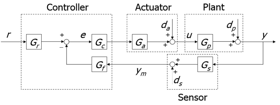
Fig 1 : Block diagram of the control system
I think everything is clear here (di - disturbances).
Problem statement:
Find : Gc (s) and Gf (s) which satisfy all given conditions.
Given: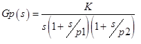 - control object with uncertainties that are set by intervals: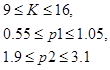
For further calculations, we will use nominal values, and we will take into account uncertainties further.
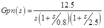
Kn = (16 + 9) /2=12.5,p1n=0.8,p2n=2.5 , respectively, received the nominal control object:

Types of disturbances:
Or in other words, these are the noise characteristics of system elements.
I will not paint in very detail, only the main points.
One of the key steps in the H∞ method is the definition of input and output weight functions. These weighting functions are used to normalize the input and output and reflect the time and frequency dependences of the input disturbances and the operating characteristics of the output variables (errors) [1]. Honestly, it practically doesn’t mean anything to me, especially if this is the first time you encounter this method. In a nutshell, weight functions are used to set the desired properties of the control system. For example, in the feedback there is a sensor that has noise, usually high-frequency, and so, the weight function will be a kind of boundary that the controller should not cross in order to filter out the sensor noise.
Below we will derive these weight functions based on performance.
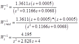
As a result, we get:
The Hinf method or the method of minimizing the infinite norm Hinfinity refers to the general formulation of the control problem, which is based on the following feedback control system representation diagram:
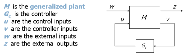
Fig. 12 : Generalized control system diagram
Let us go to the controller calculation point and what is needed for this. They didn’t explain the study of calculation algorithms to us, they said: “Do this and it will work out”, but the principle is quite logical. The controller is obtained in the course of solving the optimization problem:

 - a closed transfer function from W to Z.
Now we need to make a generalized plant (dashed rectangle pic below). Gpn we have already identified, this is a nominal control object. Gc - the controller that we get in the end. W1 = Ws (s), W2 = max (WT (s), Wu (s)) are the weight functions defined earlier. Wu (s) is the weight function of uncertainty, let's define it.
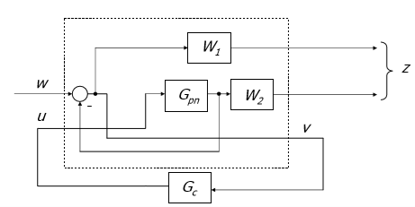
Figure 13 : Disclosed Control Schemes
Suppose that we have multiplicative uncertainties in the control object, we can depict this:
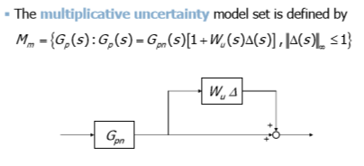
Fig. 14 : Multiplicative uncertainty.
And so, to find Wu, we use the matlab. We need to build Bode all possible deviations from the nominal control object, and then build the transfer function that will describe all these uncertainties:
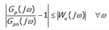
We will make about 4 passes for each parameter and build a bode. As a result, we get this:
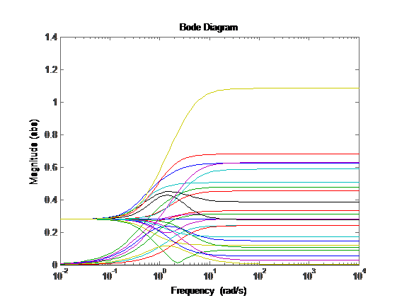
Figure 15 : The Bode digest of uncertainties
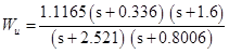
Wu will lie above these lines. The matlab has a tool that allows you to use the mouse to indicate points and builds a transfer function from these points.
After entering the points, the curve ages and it is proposed to introduce the degree of the transfer function, we introduce the degree of 2.
Here's what happened:
Now we define W2, for this we construct Wt and Wu:
From the graph it is clear that Wt is greater than Wu means W2 = Wt.
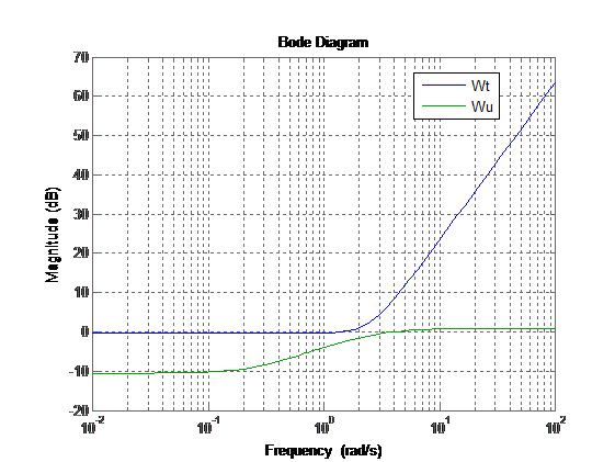
Figure 16 : Definition of W2
Next, we need to build a generalized plant in simulink as follows:
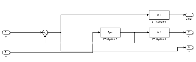
Figure 17 : Block diagram of the Generalized plant in simulink
And save it under the name, for example g_plant.mdl
One important point:
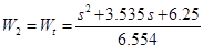 - not proper tf, if we leave it like that we will get an error. Therefore, replace with
  and then add two zeros to the output of z2 using “sderiv“.
After executing this code, we get the controller:

In principle, you can leave it that way, but usually low- and high-frequency zeros and poles are deleted. Thus, we reduce the order of the controller. And we get the following controller:

we get such a Hichols chart:
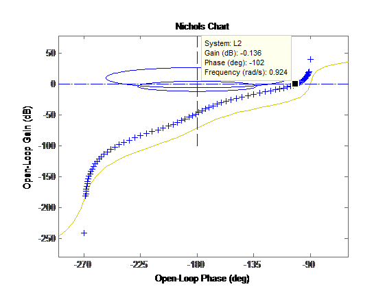
Figure 18 : Hichols chart of an open system with the resulting controller
And Step response:
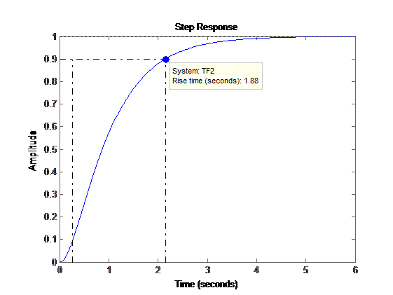
Figure 19 : Transient response of the closed system with the controller
And now the sweetest thing. Whether our controller turned out robust or not. For this experiment, we just need to change our control object (coefficients k, p1, p2) and see the step response and the characteristics of interest, in our case it is overshoot, regulation time for 5% and rise time [2].

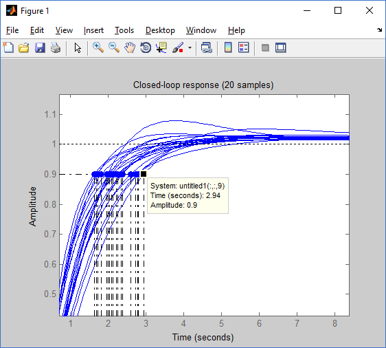
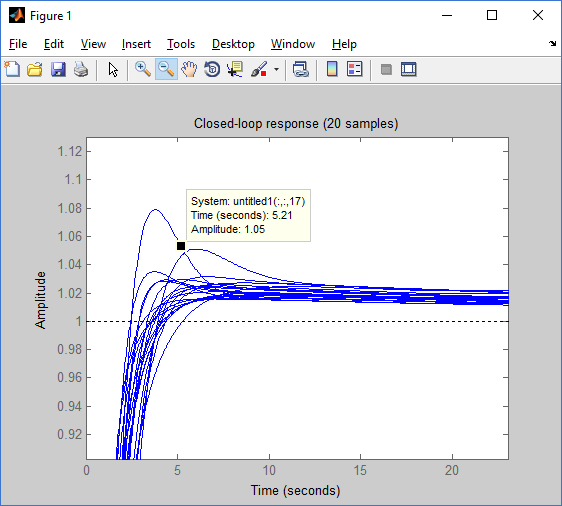
Fig 20: Temporal characteristics for different parameters of the control object
Having built 20 different transient characteristics, I identified the maximum values for each temporal characteristic:
• Maximum re-adjustment - 7.89%
• Max rise time - 2.94 sec
• Max recovery time 5% - 5.21 sec
And oh miracle, characteristics where necessary not only for the nominal object, but also for the parameter interval.
Now, let's compare it with the classic PID controller, and let's see if the game was worth the candle or not.
PID calculated pidtool for the nominal control object (see above):
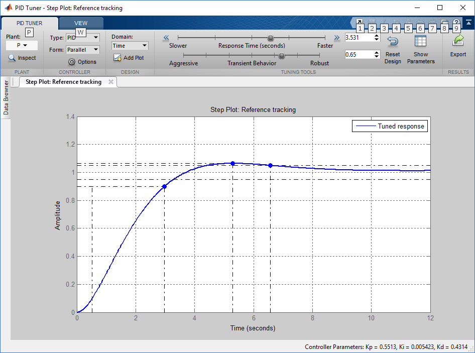
Fig. 21 : Pidtool.
We will get such a controller:
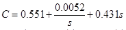
Now H-infinity vs PID :
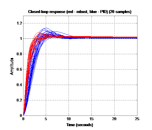
Fig. 22: H-infinity vs PID
It is clear that the PID can not cope with such uncertainties and the PX goes beyond the given limits, while the robust controllers “rigidly” keep the system in the given intervals of overshoot, rise time and regulation.
In order not to lengthen the article and not bore the reader, I will omit the verification of characteristics 2-5 (errors), I will say that in the case of a robust controller all errors are below the set, a test was also conducted with other parameters of the object:
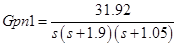
Errors were below the set, which means That this controller fully copes with the task. While the PID could not cope only with paragraph 4 (dp error).
That's all for the calculation of the controller. Criticize, ask.
Link to the matlab file:drive.google.com/open?id=0B2bwDQSqccAZTWFhN3kxcy1SY0E
1. Guidelines for the Selection of Weighting Functions for H-Infinity Control
2. it.mathworks.com/help/robust/examples/robustness-of-servo-controller-for-dc-motor.html
The answer lies in the title itself, from English. “Robustness” - The quality of being strong and not easy to break. In the case of the controller, this means that it must be “tough”, resistant to changes in the control object. For example: in mat. DC motor models have 3 main parameters: the resistance and inductance of the winding, and the constant Кт Ке, which are equal to each other. To calculate the classic PID controller, look at the datasheet, take those 3 parameters and calculate the PID coefficients, everything seems to be simple, what else is needed. But the motor is a real system in which these 3 coefficients are not constant, for example, as a result of high-frequency dynamics, which is difficult to describe or requires a high order of the system. for instance: Rdatashit = 1 Ohm, but in fact, R is in the range [0.9,1.1] Ohm. So in the case of quality indicators in the case of the PID controller, they can go beyond the set ones, and the robust controller takes into account uncertainties and is able to keep the quality indicators of a closed system in the right interval.
At this stage, a logical question arises: How to find this interval? It is found using the parametric identification of the model. On Habré recently described the method of OLS ( "Parametric identification of a linear dynamic system" ), however, it gives one value of the identifiable parameter, as in a datasheet. To find the range of values, we used the Sparse Semide Finite Programming Relaxation of Polynomial Optimization Problems»Supplement for matlaba. If it is interesting, I can write a separate article how to use this package and how to make identification.
I hope that now it is at least not much clearer why robust control is needed.
I will not particularly go into theory, because I did not quite understand it; I will show the steps that you need to go through to get the controller. If you're interested, check out the Essentials Of Robust Control, Kemin Zhou, John C. Doyle, Prentice Hall, or the Matlab documentation.
We will use the following control system diagram:
Fig 1 : Block diagram of the control system
I think everything is clear here (di - disturbances).
Problem statement:
Find : Gc (s) and Gf (s) which satisfy all given conditions.
Given:
- control object with uncertainties that are set by intervals: For further calculations, we will use nominal values, and we will take into account uncertainties further.
Kn = (16 + 9) /2=12.5,p1n=0.8,p2n=2.5 , respectively, received the nominal control object:
Types of disturbances:
 - stepwise disturbance of the amplifier with amplitude D_a0
 - sinusoidal disturbance of the control object with amplitude a_p and frequency w_p
 - sinusoidal disturbance of the sensor with amplitude a_s and frequency w_s
Or in other words, these are the noise characteristics of system elements.
Performance specifications
- Gain of the control system Kd = 1
- Steady-state error at input impact Ramp R0 = 1:

- The established error in the presence of da:

- Steady error in the presence of dp:

- Steady error in the presence of ds:

- Overshoot

- Regulation time

- Rise time

Decision
I will not paint in very detail, only the main points.
One of the key steps in the H∞ method is the definition of input and output weight functions. These weighting functions are used to normalize the input and output and reflect the time and frequency dependences of the input disturbances and the operating characteristics of the output variables (errors) [1]. Honestly, it practically doesn’t mean anything to me, especially if this is the first time you encounter this method. In a nutshell, weight functions are used to set the desired properties of the control system. For example, in the feedback there is a sensor that has noise, usually high-frequency, and so, the weight function will be a kind of boundary that the controller should not cross in order to filter out the sensor noise.
Below we will derive these weight functions based on performance.
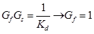 Everything is simple here.
- In this paragraph, we need to determine how many poles at zero it is necessary for the controller (we denote µ) to satisfy Condition 2. To do this, we use the table:
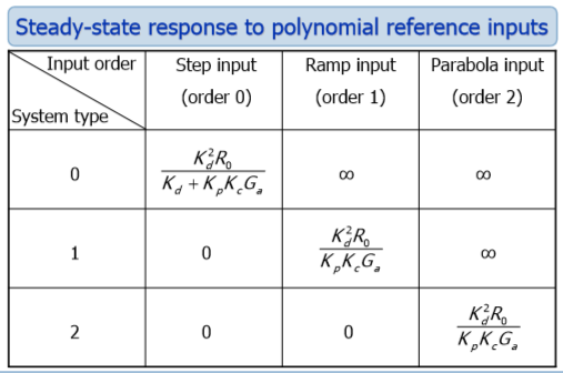
Fig 2 : Errors in position, speed and acceleration
System type or astatism (p) - indicates the number of poles in zero, of the control object, in our case p = 1 (a system with first-order astatism). Since our control object is a system with first-order astatism, in this case the controller should not have poles at zero. We use the formula:
μ + p = h
Where h is the order of the input signal, for ramp h = 1;
μ = hp = 1-1 = 0
Now we use the finite value theorem to find e_r∞
where e_r is the tracking error,
yr is the actual output (see Figure 1), yd is the desired output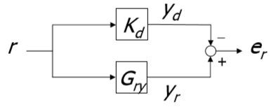
Figure 3 : Determining the tracking error
As a result, we get this:
This is the steady-state error formula unknown in this equation S (Sensitivity function)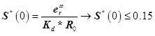
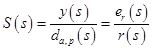
Where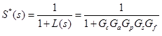 - sensitivity function, L (s) - loop function. Without a clue how they are translated into Russian, I will leave the English names. Also, complementary sensitivity function
 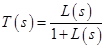 (as seen from the formulas, S and T include Gc - the calculated controller, respectively, we find the boundaries for S and T from errors and performance characteristics, we determine the weight functions from S and T, and the matlab from the weight functions will find controller.)
In a nutshell about S and T [1].- Sensitivity function , S (s), describes the output y (s) as a function of the disturbance da and dp, also relates the tracking error and the input action (for low frequencies)
- Complementary sensitivity function , T (s), connects the system output with the input action, and also shows how much sensor noise ds affects the system output (for high frequencies).
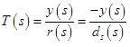
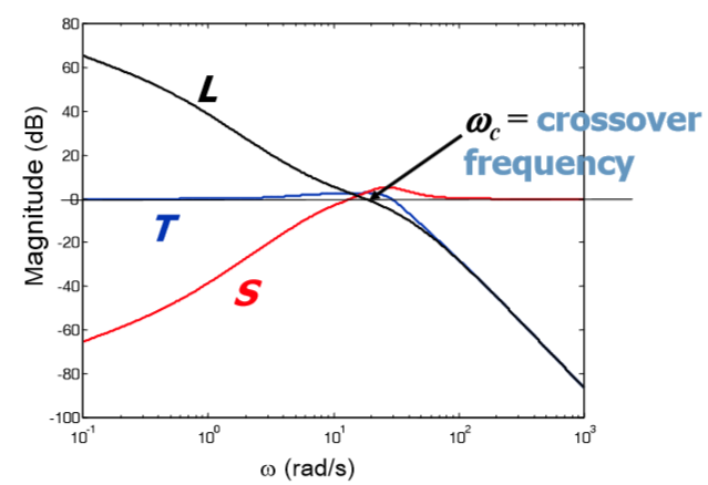
Figure 4 : Bode diagram for S, T, and L.
From the graph it can be seen that S attenuates the low-frequency disturbances, while T attenuates the high-frequency disturbances. - Sensitivity function , S (s), describes the output y (s) as a function of the disturbance da and dp, also relates the tracking error and the input action (for low frequencies)
- We use the finite value theorem for e_da

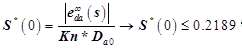
Since we have two inequalities, we find a condition satisfying both:
This condition says where the Sensitivity function should intersect the 0 dB axis in the Bode diagram.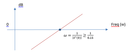
Figure 5 : Bode for S - Dp, we have a harmonic perturbation, low-frequency. Create a mask for S in the frequency region wp
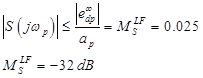
This value shows that S must be below -32 dB for frequencies wp to filter out disturbances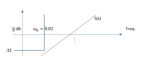
Fig. 6 : Mask for S - Ds is also a harmonic disturbance of high frequencies, here T will play its role.
Do the same: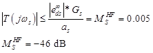
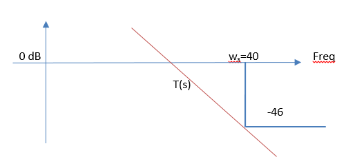
Figure 7 : Mask for T
The complex order of weight functions is determined from the mask condition and the frequency of intersection with the 0 axis. In our case, from wp to w is about one decade, and since we have -32 dB, then S must be at least 2 orders of magnitude. The same applies to T.
As a result, the restriction diagrams are as follows for S and T, respectively: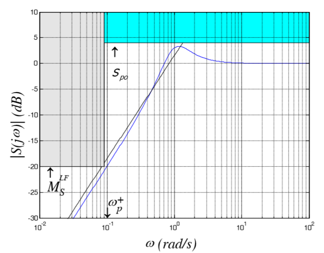
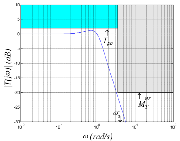
Figure 8 : All masks for S and T - To translate the time characteristics, we use the graphs
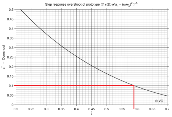
Fig. 9 : Graph of the damping coefficient versus re-adjustment
Knowing the re-adjustment we find the damping coefficient for 10% ->
ξ = 0.59
Knowing the damping coefficient we find the (resonant) maximum value for S and T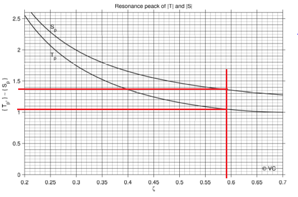
Fig. 10 : S_p0 and T_p0 dependence from damping coefficient S_p0
= 1.35
T_p0 = 1.05 - From the time of regulation and tuning, we find how fast the control system should be.

Next, we find the natural frequency for S The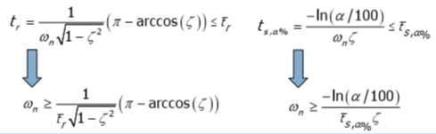

natural frequency for T is found from the Bode diagram. According to condition 5, at a frequency of 40 rad / s, T should be below -46 dB, which means that with a slope of -40 dB / dec, the natural frequency should be below 4 rad / s. Building the Bode, we select the optimal value, I got that:
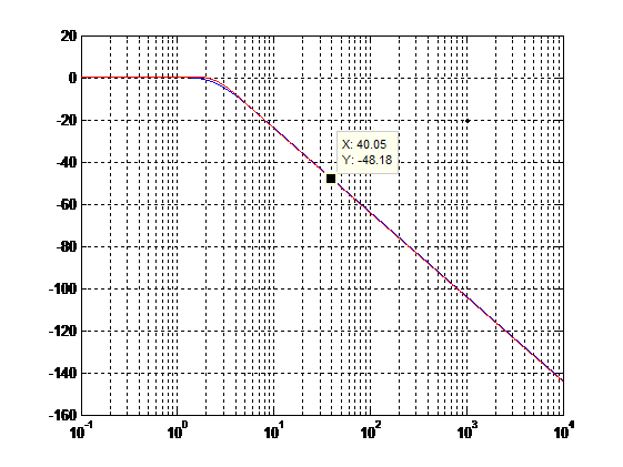
Figure 11 : Bode T-functions
After that, we have all the data for constructing the ST, which we then transform into weighted functions. ST have the following form: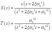
Normally to build weighting functions used Butterworth coefficients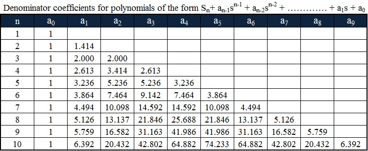
weighting functions have the form: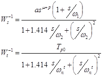
For simple, and we have everything you need, which would be substituted into the formula. For
 some more calculations are needed.
Since the performance characteristics give us the boundary conditions under which our controller will fulfill all conditions. Weighting functions combine all conditions and then are used as the right and left boundaries in which the controller is located that satisfies all conditions.
For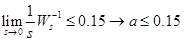 this parameter is called generalized DC gain, it displays the behavior for low frequencies (s = 0)
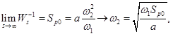 , w1, we choose approximately near the perturbation frequency or one decade below (set to 0.0005 rad / s)
- • LMI solver does not accept function zeros (zero in origine), therefore we replace s with zero near the origin (s + 0.0005)
As a result, we get:
Generalized plant
The Hinf method or the method of minimizing the infinite norm Hinfinity refers to the general formulation of the control problem, which is based on the following feedback control system representation diagram:
Fig. 12 : Generalized control system diagram
Let us go to the controller calculation point and what is needed for this. They didn’t explain the study of calculation algorithms to us, they said: “Do this and it will work out”, but the principle is quite logical. The controller is obtained in the course of solving the optimization problem:
- a closed transfer function from W to Z.Now we need to make a generalized plant (dashed rectangle pic below). Gpn we have already identified, this is a nominal control object. Gc - the controller that we get in the end. W1 = Ws (s), W2 = max (WT (s), Wu (s)) are the weight functions defined earlier. Wu (s) is the weight function of uncertainty, let's define it.
Figure 13 : Disclosed Control Schemes
Wu (s)
Suppose that we have multiplicative uncertainties in the control object, we can depict this:
Fig. 14 : Multiplicative uncertainty.
And so, to find Wu, we use the matlab. We need to build Bode all possible deviations from the nominal control object, and then build the transfer function that will describe all these uncertainties:
We will make about 4 passes for each parameter and build a bode. As a result, we get this:
Figure 15 : The Bode digest of uncertainties
Wu will lie above these lines. The matlab has a tool that allows you to use the mouse to indicate points and builds a transfer function from these points.
Code
mf = ginput(20);
magg = vpck(mf(:,2),mf(:,1));
Wa = fitmag(magg);
[A,B,C,D]=unpck(Wa);
[Z,P,K]=ss2zp(A,B,C,D);
Wu = zpk(Z,P,K)
magg = vpck(mf(:,2),mf(:,1));
Wa = fitmag(magg);
[A,B,C,D]=unpck(Wa);
[Z,P,K]=ss2zp(A,B,C,D);
Wu = zpk(Z,P,K)
After entering the points, the curve ages and it is proposed to introduce the degree of the transfer function, we introduce the degree of 2.
Here's what happened:
Now we define W2, for this we construct Wt and Wu:
From the graph it is clear that Wt is greater than Wu means W2 = Wt.
Figure 16 : Definition of W2
Next, we need to build a generalized plant in simulink as follows:
Figure 17 : Block diagram of the Generalized plant in simulink
And save it under the name, for example g_plant.mdl
One important point:
- not proper tf, if we leave it like that we will get an error. Therefore, replace with and then add two zeros to the output of z2 using “sderiv“.Implementation in Matab
p = 2; % частота нулей в районе частоты Т функции
[Am,Bm,Cm,Dm] = linmod('g_plant');
M = ltisys(Am,Bm,Cm,Dm);
M = sderiv(M,2,[1/p 1]);
M = sderiv(M,2,[1/p 1]);
[gopt,Gcmod] = hinflmi(M,[1 1],0,0.01,[0,0,0]);
[Ac,Bc,Cc,Dc] = ltiss(Gcmod);
[Gc_z,Gc_p,Gc_k] = ss2zp(Ac,Bc,Cc,Dc);
Gc_op = zpk(Gc_z,Gc_p,Gc_k)
[Am,Bm,Cm,Dm] = linmod('g_plant');
M = ltisys(Am,Bm,Cm,Dm);
M = sderiv(M,2,[1/p 1]);
M = sderiv(M,2,[1/p 1]);
[gopt,Gcmod] = hinflmi(M,[1 1],0,0.01,[0,0,0]);
[Ac,Bc,Cc,Dc] = ltiss(Gcmod);
[Gc_z,Gc_p,Gc_k] = ss2zp(Ac,Bc,Cc,Dc);
Gc_op = zpk(Gc_z,Gc_p,Gc_k)
After executing this code, we get the controller:
In principle, you can leave it that way, but usually low- and high-frequency zeros and poles are deleted. Thus, we reduce the order of the controller. And we get the following controller:
we get such a Hichols chart:
Figure 18 : Hichols chart of an open system with the resulting controller
And Step response:
Figure 19 : Transient response of the closed system with the controller
And now the sweetest thing. Whether our controller turned out robust or not. For this experiment, we just need to change our control object (coefficients k, p1, p2) and see the step response and the characteristics of interest, in our case it is overshoot, regulation time for 5% and rise time [2].
Fig 20: Temporal characteristics for different parameters of the control object
Having built 20 different transient characteristics, I identified the maximum values for each temporal characteristic:
• Maximum re-adjustment - 7.89%
• Max rise time - 2.94 sec
• Max recovery time 5% - 5.21 sec
And oh miracle, characteristics where necessary not only for the nominal object, but also for the parameter interval.
Now, let's compare it with the classic PID controller, and let's see if the game was worth the candle or not.
PID calculated pidtool for the nominal control object (see above):
Fig. 21 : Pidtool.
We will get such a controller:
Now H-infinity vs PID :
Fig. 22: H-infinity vs PID
It is clear that the PID can not cope with such uncertainties and the PX goes beyond the given limits, while the robust controllers “rigidly” keep the system in the given intervals of overshoot, rise time and regulation.
In order not to lengthen the article and not bore the reader, I will omit the verification of characteristics 2-5 (errors), I will say that in the case of a robust controller all errors are below the set, a test was also conducted with other parameters of the object:
Errors were below the set, which means That this controller fully copes with the task. While the PID could not cope only with paragraph 4 (dp error).
That's all for the calculation of the controller. Criticize, ask.
Link to the matlab file:drive.google.com/open?id=0B2bwDQSqccAZTWFhN3kxcy1SY0E
List of references
1. Guidelines for the Selection of Weighting Functions for H-Infinity Control
2. it.mathworks.com/help/robust/examples/robustness-of-servo-controller-for-dc-motor.html