How a programmer bought a car
Recently, I was puzzled by the search for used car, instead of just sold, and, as is usually the case, several competitors claimed this role.
As you know, to buy a car in the Russian Federation there are several large reputable sites (auto.ru, drom.ru, avito.ru), for which I gave preference to search. Hundreds, and for some models and thousands, of cars, from the sites listed above met my requirements. Besides the fact that it’s inconvenient to search on several resources, before going to watch a car “live”, I would like to select the advantageous (the price of which is lower than the market) offers for a priori information that each of the resources provides. Of course, I really wanted to solve several overdetermined systems of algebraic equations (possibly non-linear) of high dimension manually, but I overpowered myself and decided to automate this process.

I collected data from all the resources described above, and I was interested in the following parameters:
Unfilled lazy sellers details I noted as an NA (Not Available), to be able to correctly handle these values using the R .
In order not to go into dry theory, let's look at a specific example, we will look for profitable Mercedes-Benz E-class no older than 2010 release, costing up to 1.5 million rubles in Moscow. In order to start working with data, first of all, fill in the missing values (NA) with median values, fortunately there is a median () function in R for this.
For the remaining variables, the procedure is identical, so I will omit this point.
Now let's see how the price depends on the regressors (we are not interested in visualizing indicator variables at this stage).
It turns out for this money there are several cars in 2013 and even one in 2014!
Obviously, the lower the mileage, the higher the price.

On some of the graphs, we see points that stand out from the general sample - emissions , excluding which, we can make an assumption about the linear dependence of the price on the vehicle parameters.
I want to draw your attention to the fact that in most of the articles on machine learning that have come to me recently, including on “Habré”, very little attention is paid to the justification of the legitimacy of using the selected model, its diagnostics, and errors.
Therefore, in order for the estimates obtained by us to be consistent, it is reasonable to consider the issue of the correctness of our chosen model.
In the previous section, on the basis of experimental data, an assumption was made about the linearity of the model under consideration with respect to price, so in this section we will talk about multiple linear regression , its diagnosis and errors.
For the model to be correct, it is necessary to fulfill the conditions of the Gauss-Markov theorem :
So, the time has come when the bureaucracy is over, the correctness of using the linear regression model is beyond doubt. We can only calculate the coefficients of the linear equation by which we can get our predicted car prices and compare them with the prices from the ads.
And now, let's collect all the research done in a heap, for the sake of one of the most informative graphs, which will show us the most desirable value for any automobile reseller, the value of the benefit from buying a particular car relative to the market price.
And what percentage benefit can you expect?
Yes, saving 59% is very cool, but very doubtful, you need to watch a car “live”, because free cheese is usually in a mousetrap, well, or the seller urgently needs money. But starting from 4th place (saving 28%) and further, the result seems quite realistic.
I would like to draw attention to the fact that the coefficients of the linear model are formed by measurements with excluded emissions, to reduce the error of predictive analysis, while we predict the price for all offers on the market, which undoubtedly increases the probability of an error in predicting the price for emissions (for example, as in In our case, all cars with a station wagon body may fall into emissions, as a result of which, the correction, which the corresponding indicator variable should make, is not taken into account), which is a drawback of the selected model . Of course, you can not predict the price for offers that are very different from the total sample, but it is highly likely that among them are the most advantageous offers.
Dear friends, I myself, having read a similar article, would have asked primarily 3 questions:
Therefore, I answer:
1. Source data in csv format - dataset.txt
As you know, to buy a car in the Russian Federation there are several large reputable sites (auto.ru, drom.ru, avito.ru), for which I gave preference to search. Hundreds, and for some models and thousands, of cars, from the sites listed above met my requirements. Besides the fact that it’s inconvenient to search on several resources, before going to watch a car “live”, I would like to select the advantageous (the price of which is lower than the market) offers for a priori information that each of the resources provides. Of course, I really wanted to solve several overdetermined systems of algebraic equations (possibly non-linear) of high dimension manually, but I overpowered myself and decided to automate this process.
Data collection
I collected data from all the resources described above, and I was interested in the following parameters:
- price
- year of manufacture (year)
- mileage
- engine volume (engine.capacity)
- engine power (engine.power)
- engine type (2 indicator mutually exclusive variables diesel and hybrid, taking values 0 or 1, for diesel and hybrid engines, respectively). The default engine type is gasoline (not moved to the third variable to avoid multicollinearity ).
Thus: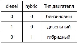
Further, similar logic for indicator variables is implied by default. - gearbox type (indicator variable mt (manual transmission), which takes a Boolean value, for a manual transmission). The default gearbox type is automatic.
It should be noted that I attributed to automatic transmissions not only a classic hydraulic machine, but also robotic mechanics and a variator. - drive type (2 indicator variables front.drive and rear.drive accepting Boolean values). The default drive type is full.
- body type (7 indicator variables sedan, hatchback, wagon, coupe, cabriolet, minivan, pickup, taking Boolean values). The default body type is SUV / Crossover
Unfilled lazy sellers details I noted as an NA (Not Available), to be able to correctly handle these values using the R .
Data visualization
In order not to go into dry theory, let's look at a specific example, we will look for profitable Mercedes-Benz E-class no older than 2010 release, costing up to 1.5 million rubles in Moscow. In order to start working with data, first of all, fill in the missing values (NA) with median values, fortunately there is a median () function in R for this.
dat <- read.csv("dataset.txt") # загружаем выборку в R
dat$mileage[is.na(dat$mileage)] <- median(na.omit(dat$mileage)) # например для пробега
For the remaining variables, the procedure is identical, so I will omit this point.
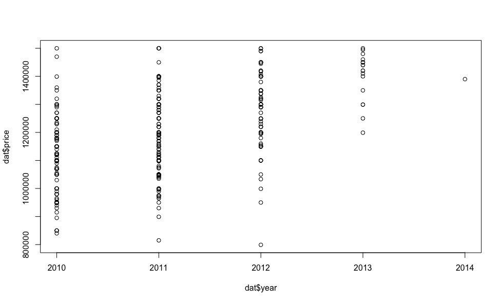
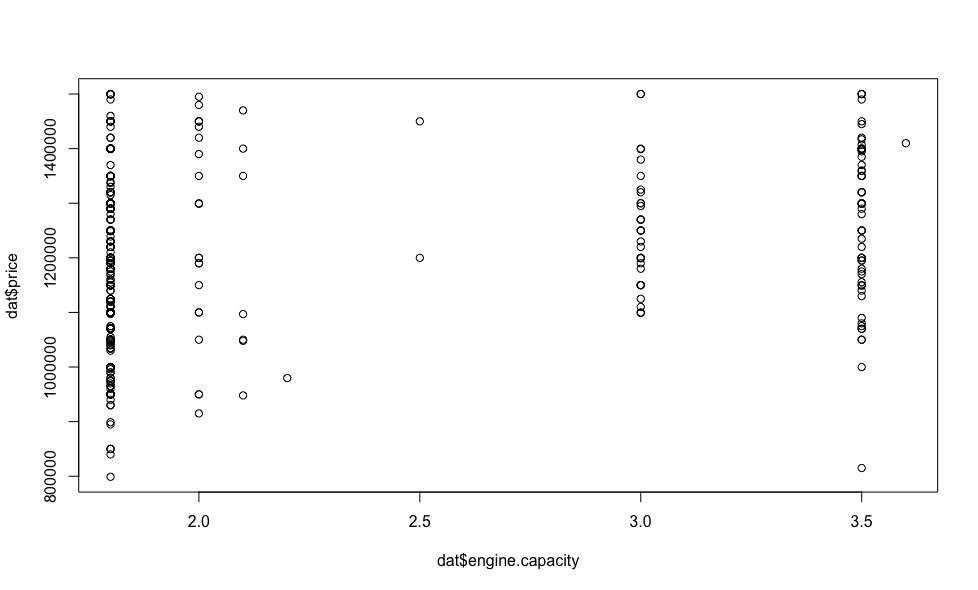
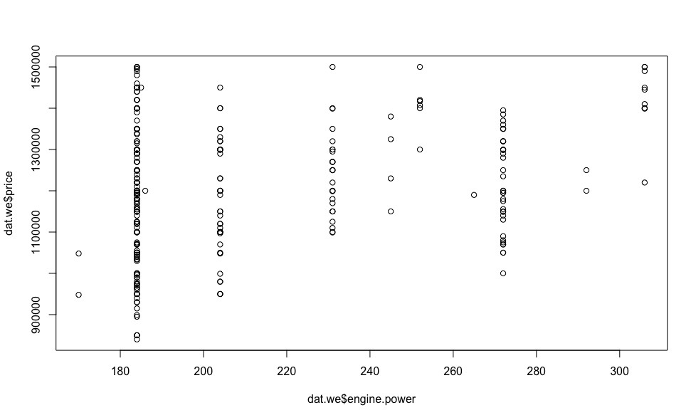
Now let's see how the price depends on the regressors (we are not interested in visualizing indicator variables at this stage).
It turns out for this money there are several cars in 2013 and even one in 2014!
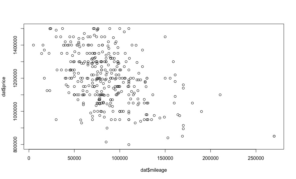
Obviously, the lower the mileage, the higher the price.
On some of the graphs, we see points that stand out from the general sample - emissions , excluding which, we can make an assumption about the linear dependence of the price on the vehicle parameters.
I want to draw your attention to the fact that in most of the articles on machine learning that have come to me recently, including on “Habré”, very little attention is paid to the justification of the legitimacy of using the selected model, its diagnostics, and errors.
Therefore, in order for the estimates obtained by us to be consistent, it is reasonable to consider the issue of the correctness of our chosen model.
Model Diagnostics
In the previous section, on the basis of experimental data, an assumption was made about the linearity of the model under consideration with respect to price, so in this section we will talk about multiple linear regression , its diagnosis and errors.
For the model to be correct, it is necessary to fulfill the conditions of the Gauss-Markov theorem :
- The data model is correctly specified, i.e.:
- missing missing values. More detailsThis condition is fulfilled (see the Visualization of the obtained data section), the missing values are replaced by the median ones.
- there is no multicollinearity between the regressors.More detailsCheck if this condition is met:
dat_cor <- as.matrix(cor(dat)) # рассчет корреляции между переменными
dat_cor[is.na(dat_cor)] <- 0 # заменяем пропущенные значения на 0 (т.к. например в кузове пикап или минивен искомого авто не бывает)
library(corrplot) # подключаем библиотеку corrplot, для красивой визуализации
palette <-colorRampPalette(c("#7F0000","red","#FF7F00","yellow","#7FFF7F", "cyan", "#007FFF", "blue","#00007F"))
corrplot(dat_cor, method="color", col=palette(20), cl.length=21,order = "AOE", addCoef.col="green") # рисуем таблицу зависимостей между переменными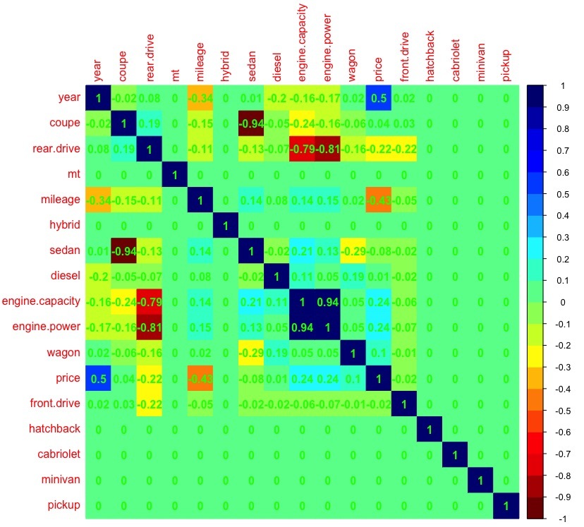
It can be seen that there is a large correlation (> 0.7) between the volume and power of the engine, therefore, in further analysis, we will not take into account the variable engine.capacity, because it is the engine power that will allow us to more accurately build a regression model compared to the engine capacity (atmospheric gasoline, turbocharged gasoline, diesel engines - with the same volume, they can have different power). - no emissions .More detailsEmissions - indicators allocated from the general sample (see the Visualization of the data obtained section), have a significant impact on the estimates of the coefficients of the regression model. A statistical method that can operate under outlier conditions is called robust - linear regression does not apply to them, unlike, for example, the Huber robust regression or the truncated squares method.
Measures of the impact of emissions on model estimates can be divided into general and specific. General measures, such as Cook distance, dffits, covariacin ratio (covratio), Mahalanobis distance, show how the i-th observation affects the position of the entire regression dependence, and we will use them to identify outliers. Specific measures of influence, such as dfbetas, show the influence of the ith observation on the individual parameters of the regression model.
Covariacin ratio (covratio) is a common measure of the effect of observation. It is the ratio of the determinant of the covariance matrix with the remote i-th observation to the determinant of the covariance matrix for the entire data set.
The Cook distance is a quadratic dependence on the internal studentized residue, which is not recommended for outlier detection, in contrast to the external studentized residue, on which dffits linearly depends.
The distance of Mahalanobis is a measure of the removal of observation from the center of the system, but because it does not take into account the dependent or independent nature of the variable and treats them equally in the scattering cloud; this measure is not intended for regression analysis.
Thus, we will use dffits and covratio measures to detect emissions.model <- lm(price ~ year + mileage + diesel + hybrid + mt + front.drive + rear.drive + engine.power + sedan + hatchback + wagon + coupe + cabriolet + minivan + pickup, data = dat) # линейная модель model.dffits <- dffits(model) # рассчитаем меру dffits
Significant for the dffits measure are indicators that exceed 2 * sqrt (k / n) = 0.42, so you should discard them (k is the number of variables, n is the number of rows in the sample).model.dffits.we <- model.dffits[model.dffits < 0.42] model.covratio <- covratio(model) # рассчитаем ковариационное отношения для модели
Significant measures for covratio measures can be found from inequality | model.covratio [i] -1 | > (3 * k) / n.model.covratio.we <- model.covratio[abs(model.covratio -1) < 0.13] dat.we <- dat[intersect(c(rownames(as.matrix(model.dffits.we))), c(rownames(as.matrix(model.covratio.we)))),] # наблюдения без выбросов model.we <- lm(price ~ year + mileage + diesel + hybrid + mt + front.drive + rear.drive + engine.power + sedan + hatchback + wagon + coupe + cabriolet + minivan + pickup, data = dat.we) # линейная модель построенная по выборке без выбросов
And now, after removing the observations that stand out from the general sample, let's look at the graphs of the dependence of the price on the regressors.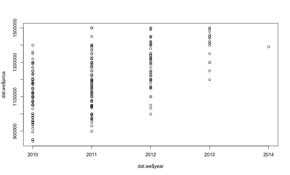

In total, the chosen method for identifying outliers allowed us to exclude 18 observations from the total sample, which will undoubtedly positively affect the accuracy of determining the coefficients of the linear model using OLS .
- missing missing values.
- All regressors are deterministic and not equal.More detailsThis condition is met.
- Errors are not systematic, the variance of errors is the same ( homoskedasticity )More detailsLet's see how the model errors are distributed (to calculate the model errors in R there is a resid () function).
plot(dat.we$year, resid(model.we))
plot(dat.we$mileage, resid(model.we))
plot(dat.we$engine.power, resid(model.we))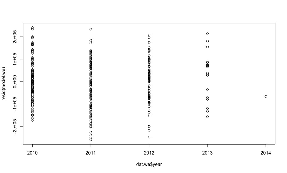
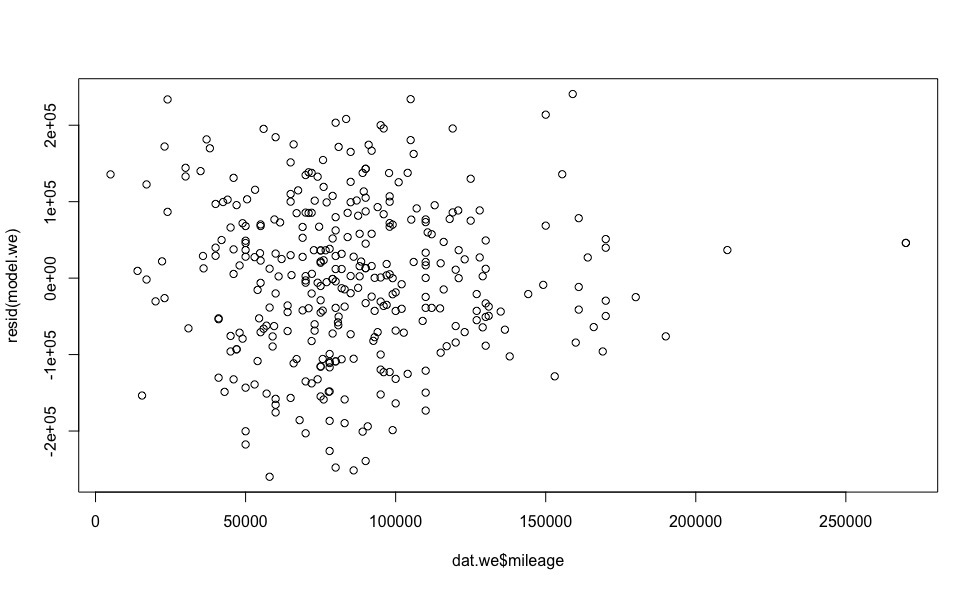
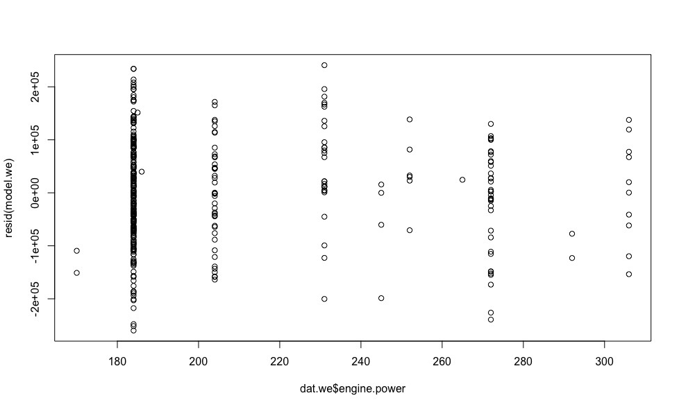
Errors are more or less evenly distributed relative to the horizontal axis, which allows us to have no doubt that the homoskedasticity condition is fulfilled. - Errors are distributed normally.More detailsTo verify this condition, we construct a graph of the quantiles of residues versus quantiles, which could be expected provided that the residues are normally distributed.
qqnorm(resid(model.we))
qqline(resid(model.we))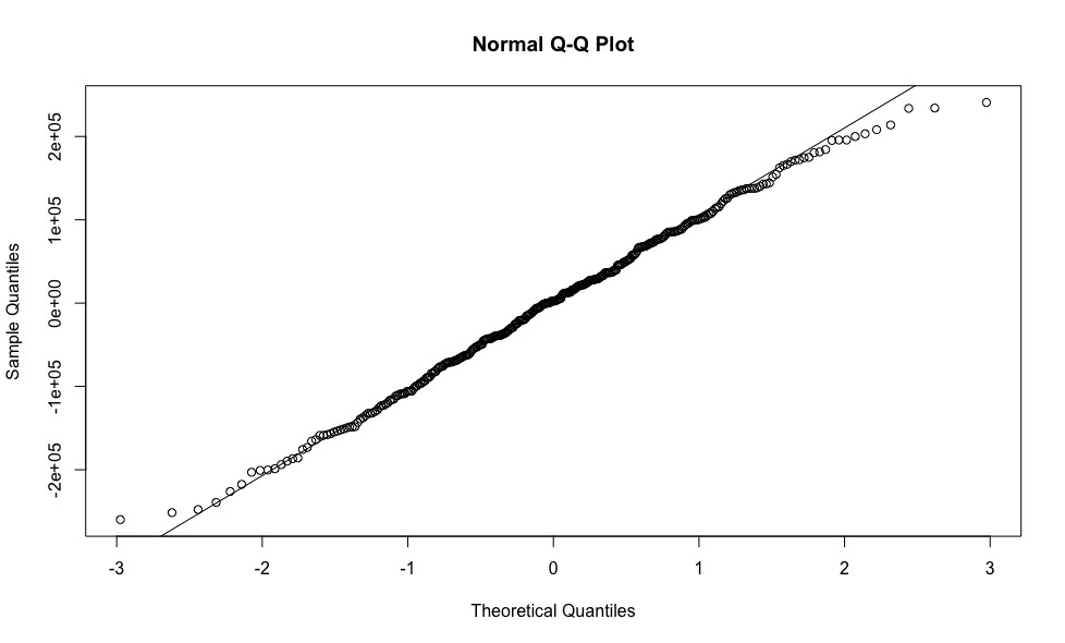
Testing the selected model
So, the time has come when the bureaucracy is over, the correctness of using the linear regression model is beyond doubt. We can only calculate the coefficients of the linear equation by which we can get our predicted car prices and compare them with the prices from the ads.
model.we <- lm(price ~ year + mileage  + diesel + hybrid + mt + front.drive + rear.drive + engine.power + sedan + hatchback + wagon + coupe + cabriolet + minivan + pickup, data = dat.we)
coef(model.we) # коэффициенты линейной модели
  (Intercept)  year  mileage  diesel  rear.drive  engine.power  sedan
  -1.76e+08  8.79e+04  -1.4e+00  2.5e+04  4.14e+04  2.11e+03  -2.866407e+04
predicted.price <- predict(model.we, dat) # предскажем цену по полученным коэффициентам
real.price <- dat$price # вектор цен на автомобили полученный из объявлений
profit <- predicted.price - real.price # выгода между предсказанной нами ценой и ценой из объявлений
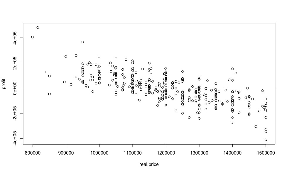
And now, let's collect all the research done in a heap, for the sake of one of the most informative graphs, which will show us the most desirable value for any automobile reseller, the value of the benefit from buying a particular car relative to the market price.
plot(real.price,profit)
abline(0,0)
And what percentage benefit can you expect?
sorted <- sort(predicted.price /real.price, decreasing = TRUE)
sorted[1:10]
      69       42      122      248      168       15      244      271      109      219
1.590489 1.507614 1.386353 1.279716 1.279380 1.248001 1.227829 1.209341 1.209232 1.204062
Yes, saving 59% is very cool, but very doubtful, you need to watch a car “live”, because free cheese is usually in a mousetrap, well, or the seller urgently needs money. But starting from 4th place (saving 28%) and further, the result seems quite realistic.
I would like to draw attention to the fact that the coefficients of the linear model are formed by measurements with excluded emissions, to reduce the error of predictive analysis, while we predict the price for all offers on the market, which undoubtedly increases the probability of an error in predicting the price for emissions (for example, as in In our case, all cars with a station wagon body may fall into emissions, as a result of which, the correction, which the corresponding indicator variable should make, is not taken into account), which is a drawback of the selected model . Of course, you can not predict the price for offers that are very different from the total sample, but it is highly likely that among them are the most advantageous offers.
In the end
Dear friends, I myself, having read a similar article, would have asked primarily 3 questions:
- What is the accuracy of the model?
- Why is the simplest linear regression chosen and where is the comparison with other models?
- Why not make a service to search for profitable cars?
Therefore, I answer:
- We will test the model according to the 80/20 scheme.
set.seed(1) # инициализируем генератор случайных чисел (для воспроизводимости)
split <- runif(dim(dat)[1]) > 0.2 # разделяем нашу выборку
train <- dat[split,] # выборка для обучения
test <- dat[!split,] # тестовая выборка
train.model <- lm(price ~ year + mileage  + diesel + hybrid + mt + front.drive + rear.drive + engine.power + sedan + hatchback + wagon + coupe + cabriolet + minivan + pickup, data = train) # линейная модель построенная по выборке для обучения
train.dffits <- dffits(train.model) # рассчитаем меру dffits
train.dffits.we <- train.dffits[train.dffits < 0.42] # удалим значимые для меры dffits показатели
train.covratio <- covratio(train.model)  # рассчитаем ковариационное отношения для модели
train.covratio.we <- model.covratio[abs(model.covratio -1) < 0.13] # удалим значимые для меры covratio показатели
train.we <- dat[intersect(c(rownames(as.matrix(train.dffits.we))), c(rownames(as.matrix(train.covratio.we)))),] # выборка для обучения без выбросов
train.model.we <- lm(price ~ year + mileage  + diesel + hybrid + mt + front.drive + rear.drive + engine.power + sedan + hatchback + wagon + coupe + cabriolet + minivan + pickup, data = train.we) # линейная модель построенная по выборке для обучения без выбросов
predictions <- predict(train.model.we, test) # проверим точность на тестовой выборке
print(sqrt(sum((as.vector(predictions - test$price))^2)/length(predictions))) # средняя ошибка прогноза цены (в рублях)
[1] 121231.5
It is a lot or a little - can be found only by comparison. - Linear regression, as one of the basics of machine learning, allows you not to be distracted by the study of the algorithm, but to completely immerse yourself in the task itself.
Therefore, I decided to divide my story into 2 (and how it goes) articles.
The next article will focus on comparing models to solve our problem in order to identify the winner. - A service was developed on this topic, which is based on the winning model, which will be discussed in the next article.
And so, what came of it - the Mercedes-Benz E-class is not older than 2010, worth up to 1.5 million rubles in Moscow .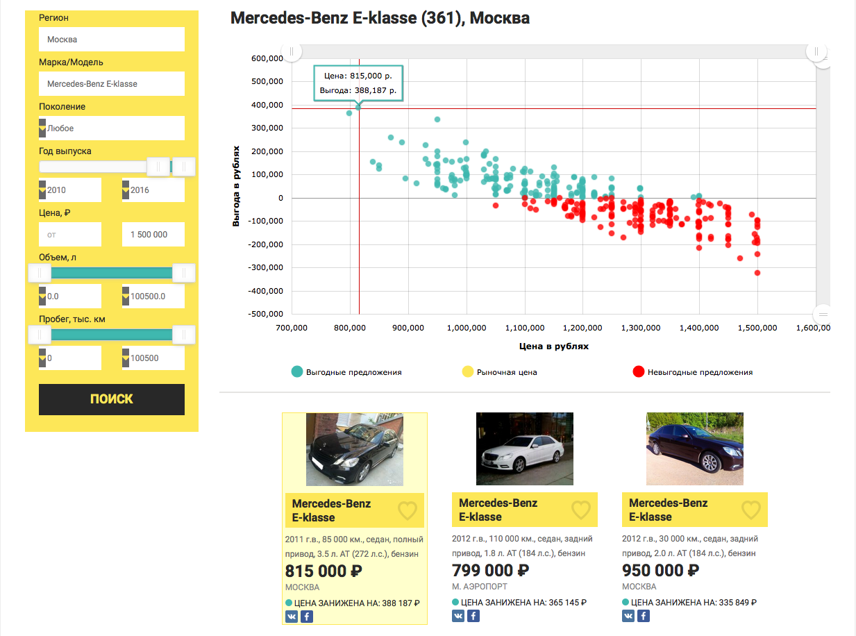 Yet
Yet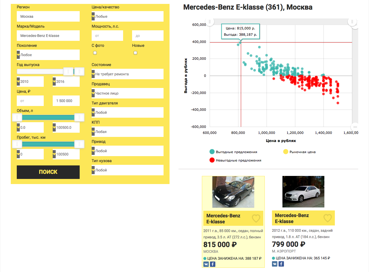
References
1. Source data in csv format - dataset.txt