Julia and phase portraits of dynamic systems

We continue to master the young and promising general-purpose language Julia . But for a start, we need just the very narrow possibility of application - for solving typical problems of physics. This is the most convenient tactic for mastering the tool: in order to fill our hands, we will solve pressing problems, gradually increasing complexity and finding ways to make our lives easier. In short, we will solve diffs and build graphs.

To begin with, download the Gadfly graphics package , and immediately the full version of the developer, so that it works well with our Julia 1.0.1. We drive in our REPL, JUNO or Jupyter notebook:

using Pkg
pkg"add Compose#master"
pkg"add Gadfly#master"

Not the most convenient option, but while waiting for the update PlotlyJS, you can compare and try.

You also need a powerful tool for solving differential equations. DifferentialEquations

]add DifferentialEquations # альтернативный способ добавления пакета

This is the most extensive and supported package, providing a lot of methods for solving difures. Now proceed to the phase portraits.

Decisions of ordinary differential equations are often more convenient to portray in a non-customary way. $$, and in the phase space , along the axes of which the values ​​of each of the functions found are deposited. In this case, the argument t is included in the graphs only parametrically. In the case of two ODEs, such a graph, the phase portrait of the system, is a curve on the phase plane and is therefore particularly intuitive.

Oscillator

Harmonic oscillator dynamics with attenuation $$ described by the following system of equations:

and regardless of the initial conditions (x0, y0), it comes to equilibrium, a point (0,0) with a zero angle of deviation and zero speed.

With $$ the decision takes the form peculiar to the classical oscillator.

using DifferentialEquations, Gadfly # включаем пакеты в проект - страшно долгий процессfunction garmosc(ω = pi, γ = 0, x0 = 0.1, y0 = 0.1)
    A = [01
        -ω^2γ]
    syst(u,p,t) = A * u # ODE system
    u0 = [x0, y0] # start cond-ns
    tspan = (0.0, 4pi) # time period
    prob = ODEProblem(syst, u0, tspan) # problem to solve
    sol = solve(prob, RK4(),reltol=1e-6, timeseries_steps = 4)
    N = length(sol.u)
    J = length(sol.u[1])
    U = zeros(N, J)
    for i in1:N, j in1:J
        U[i,j] = sol.u[i][j] # перепишем ответы в матрицу поудобнейend
    U
end

Let's sort the code. The function takes the frequency and attenuation parameter values ​​as well as the initial conditions. The nested syst () function sets the system. In order to come out single-line, they used matrix multiplication. The solve () function accepting a huge number of parameters is configured very flexibly to solve a problem, but we only indicated the method of solution — Runge-Kutta 4 ( there are many more ), the relative error, and the fact that not all points need to be saved, but only every fourth . The response matrix is ​​stored in the variable sol , and sol.t contains the vector of time values, and sol.u contains the solutions of the system at these times. All this is quietly drawn in Plots , and forGadfly will have to staff the answer in a matrix more comfortably. We do not need times, so we only return solutions.

Construct a phase portrait:

Ans0 = garmosc()
plot(x = Ans0[:,1], y = Ans0[:,2])

Among the functions of higher order for us, especially noticeable broadcast(f, [1, 2, 3]), which in the function f alternately substitutes the values ​​of the array [1, 2, 3]. A brief entry f.([1, 2, 3]). This is useful to vary the frequency, attenuation parameter, initial coordinate, and initial velocity.

L = Array{Any}(undef, 3)# создали массив чего угодно (для слоев графиков)
clr = ["red""green""yellow"]
function ploter(Answ)
    for i = 1:3
        L[i] = layer(x = Answ[i][:,1], y = Answ[i][:,2], Geom.path, Theme(default_color=clr[i]) )
    end
    p = plot(L[1], L[2], L[3])
end
Ans1 = garmosc.( [pi2pi3pi] )# частоту
p1 = ploter(Ans1)
Ans2 = garmosc.( pi, [0.10.30.5] )# затухание
p2 = ploter(Ans2)
Ans3 = garmosc.( pi, 0.1, [0.20.50.8] ) 
p3 = ploter(Ans3)
Ans4 = garmosc.( pi, 0.1, 0.1, [0.20.50.8] )
p4 = ploter(Ans4)
set_default_plot_size(16cm, 16cm)
vstack( hstack(p1,p2), hstack(p3,p4) ) # слепим горизонтально и вертикально

Now let's consider not small oscillations, but oscillations of arbitrary amplitude:

The graph of the solution on the phase plane is not an ellipse (which indicates the nonlinearity of the oscillator). The less we choose the oscillation amplitude (i.e., the initial conditions), the less non-linearity will appear (therefore, the small oscillations of the pendulum can be considered harmonic).

function ungarmosc(ω = pi, γ = 0, x0 = 0.1, y0 = 0.1)
    function syst(du,u,p,t)
        du[1] = u[2]
        du[2] = -sin( ω*u[1] )+γ*u[2]
    end
    u0 = [x0, y0] # start cond-ns
    tspan = (0.0, 2pi) # time period
    prob = ODEProblem(syst, u0, tspan) # problem to solve
    sol = solve(prob, RK4(),reltol=1e-6, timeseries_steps = 4)
    N = length(sol.u)
    J = length(sol.u[1])
    U = zeros(N, J)
    for i in1:N, j in1:J
        U[i,j] = sol.u[i][j] # перепишем ответы в матрицу поудобнейend
    U
end
Ans1 = ungarmosc.( [pi2pi3pi] )
p1 = ploter(Ans1)
Ans2 = ungarmosc.( pi, [0.10.40.7] )
p2 = ploter(Ans2)
Ans3 = ungarmosc.( pi, 0.1, [0.10.50.9] )
p3 = ploter(Ans3)
Ans4 = ungarmosc.( pi, 0.1, 0.1, [0.10.50.9] )
p4 = ploter(Ans4)
vstack( hstack(p1,p2), hstack(p3,p4) )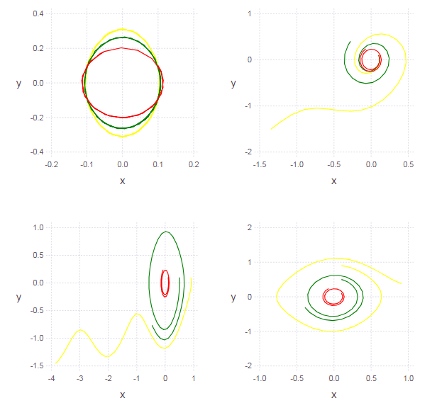

Brusselator

This model describes some autocatalytic chemical reaction in which diffusion plays a certain role. The model was proposed in 1968 by Lefebvre and Prigogine

Unknown functions $$reflect the dynamics of the concentration of intermediate products of a chemical reaction. Model parameter$$ It makes sense to the initial concentration of the catalyst (the third substance).

In more detail, the evolution of the phase portrait of the Brusselator can be observed by performing calculations with a different parameter. $$. As it increases, the node will first gradually shift to a point with coordinates (1,$$) until it reaches the bifurcation value$$= 2. At this point, a qualitative rearrangement of the portrait takes place, which is expressed in the birth of the limiting cycle. With further increase$$ there is only a quantitative change in the parameters of this cycle.

function brusselator(μ = 0.1, u0 = [0.1; 0.1])
    function syst(du,u,p,t)
        du[1] = -(μ+1)*u[1] + u[1]*u[1]*u[2] + 1
        du[2] =      μ*u[1] - u[1]*u[1]*u[2]
    end
    tspan = (0.0, 10) # time period
    prob = ODEProblem(syst, u0, tspan) # problem to solve
    sol = solve(prob, RK4(),reltol=1e-6, timeseries_steps = 1)
    N = length(sol.u)
    J = length(sol.u[1])
    U = zeros(N, J)
    for i in 1:N, j in 1:J
        U[i,j] = sol.u[i][j] # перепишем ответы в матрицу поудобней
    end
    U
end
L = Array{Any}(undef, 10)
function ploter(Answ)
    for i = 1:length(Answ)
        L[i] = layer(x = Answ[i][:,1], y = Answ[i][:,2], Geom.path )
    end
    plot(L[1], L[2], L[3], L[4], L[5], L[6], L[7], L[8], L[9], L[10])
end
SC = [ [00.5], [01.5], [2.50], [1.50], [0.51], [10], [11], [1.52], [0.10.1], [0.50.2] ]
Ans1 = brusselator.( 0.1, SC )
Ans2 = brusselator.( 0.8, SC )
Ans3 = brusselator.( 1.6, SC )
Ans4 = brusselator.( 2.5, SC )
p1 = ploter(Ans1)
p2 = ploter(Ans2)
p3 = ploter(Ans3)
p4 = ploter(Ans4)
set_default_plot_size(16cm, 16cm)
vstack( hstack(p1,p2), hstack(p3,p4) )

It's enough for today. Next time, we’ll try to learn how to use another graphic package on new tasks, at the same time getting a hand on Julia’s syntax. In the process of solving problems, they slowly begin to be traced not so directly to the pros and cons ... rather, to pleasantness and inconvenience — a separate conversation should be devoted to this. And of course, I would like to see something more serious in my games with functions — so I urge the julists to tell more about serious projects, this would help many people and me in particular in learning this wonderful language.