The book "The theoretical minimum for Big Data. All you need to know about big data

Today Big Data is big business. Information controls our life, and taking advantage of it becomes central to the work of modern organizations. No matter who you are - a business person working with analytics, a novice programmer or a developer, the “Theoretical Minimum of Big Data” will allow you not to drown in the raging ocean of modern technologies and to understand the basics of the new and rapidly developing industry of big data processing.

Want to learn about big data and how to work with it? Each algorithm is devoted to a separate chapter, which not only explains the basic principles of operation, but also gives examples of use in real-world problems. A large number of illustrations and simple comments will allow you to easily understand the most complex aspects of Big Data.

We offer you to read the excerpt "The main components"

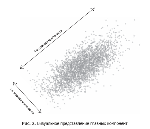
The Principal Component Analysis (CIM) method is a way to find the underlying variables (known as main components) that differentiate your data elements in an optimal way. These main components give the greatest scatter of data (Fig. 2).

The main component can express one or more variables. For example, we can use the only variable "Vitamin C". Since vitamin C is in vegetables, but not in meat, the final graph (left column in Fig. 3) will distribute the vegetables, but all the meat will be in one heap.

For the distribution of meat products, we can use fat as the second variable, since it is present in meat, but it is almost absent in vegetables. However, since fat and vitamin C are measured in different units, we must standardize them before combining them.


Standardization is the expression of each variable in percentiles that convert these variables into a single scale, allowing us to combine them to calculate a new variable:

vitamin C - fat

Since vitamin C has already distributed the vegetables up, we subtract the fat to distribute the meat down. Combining these two variables will help us distribute both vegetables and meat products (the column in the middle in Fig. 3).


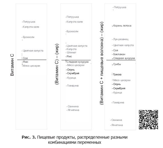
We can improve the spread, taking into account dietary fiber, the content of which in vegetables varies:

(Vitamin C + dietary fiber) - fat.

This new variable gives us the optimal data spread (right column in Fig. 3).
While we obtained the main components in this example by trial and error, the CIM can do this on a system basis. We will see how this works in the following example.

Example: food group analysis

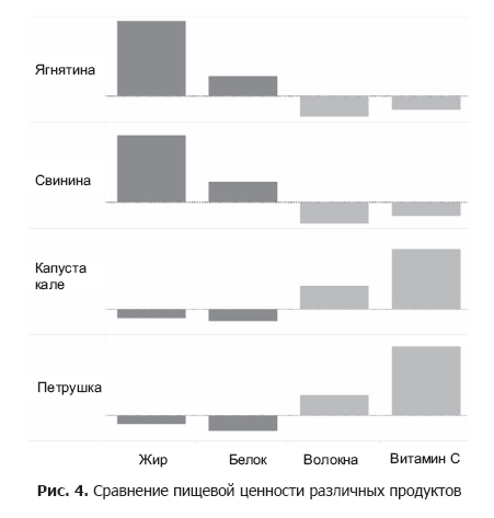
Using data from the US Department of Agriculture, we analyzed the nutritional properties of a random set of foods, examining four food variables: fats, proteins, dietary fiber, and vitamin C. As can be seen in Figure. 4, certain nutrients are often found in foods together.

In particular, the levels of fat and protein increase in one direction opposite to that in which the levels of dietary fiber and vitamin C increase. We can confirm our assumptions by checking which variables are correlated (see Section 6.5). Indeed, we find a significant positive correlation both between the levels of proteins and fats (r = 0.56), and between the levels of dietary fiber and vitamin C (r = 0.57).

Thus, instead of analyzing the four food variables separately, we can combine highly correlated ones, getting only two for consideration. Therefore, the principal component method is attributed to the techniques of decreasing dimension .


By applying it to our food data set, we get the main components shown in Figure. 5.

Each main component is a combination of food variables, the value of which can be positive, negative or close to zero. For example, to get component 1 for a single product, we can calculate the following:

.55 (dietary fiber) + .44 (Vitamin C) - .45 (fat) -
.55 (protein)


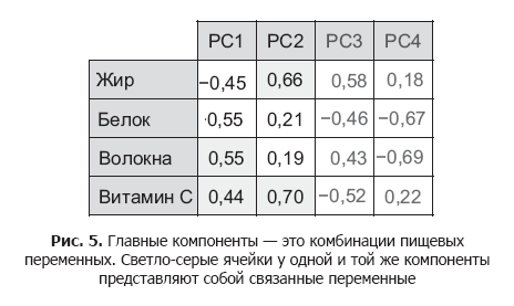
That is, instead of combining variables by trial and error, as we did before, the principal component method itself calculates the exact formulas with which you can differentiate our positions.

Please note that the main component for us, component 1 (PC1), immediately combines fats with proteins, and dietary fiber with vitamin C, and these pairs are inversely proportional.

While PC1 differentiates meat from vegetables, component 2 (PC2) more closely identifies the internal subcategories of meat (based on fat) and vegetables (based on vitamin C content). We will get the best data scattering using both components for the graph (Fig. 6).


Meat products have low components 1, therefore they are concentrated in the left part of the graph, in the opposite side from the vegetables. It is also seen that among non-vegetable products low content of fats in seafood, so the value of component 2 for them is less, and they themselves to the bottom of the graph. Similarly, for vegetables that are not green, components 2 have low values, as can be seen at the bottom of the graph to the right.

Select the number of components . In this example, four main components are created by the number of initial variables in the data set. Since the main components are created on the basis of ordinary variables, the information for the distribution of data elements is limited to their initial set.

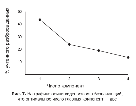
At the same time, to preserve the simplicity and scalability of the results, we should choose only the first few main components for analysis and visualization. The main components differ in the distribution efficiency of the data elements, and the first one does this to the maximum extent. The number of principal components to consider is determined using the scree chart, which we reviewed in the previous chapter.

The graph shows the decreasing efficiency of subsequent main components in the differentiation of data elements. As a rule, this number of principal components is used which corresponds to the position of an acute fracture on the scree chart.

In fig. 7 kink located at around two components. This means that while three or more major components might better differentiate data elements, this additional information may not justify the complexity of the final solution. As can be seen from the graph of scree, the first two main components already give 70% variation. Using a small number of key components for data analysis ensures that the scheme is suitable for future information.

Restrictions

The principal component method is a useful way of analyzing data sets with several variables. However, it has its drawbacks.

Maximize distribution . CIM is based on the important assumption that the most useful measurements are those that give the most variation. However, this is not always the case. A well-known counterexample is the task of counting pancakes in a stack.


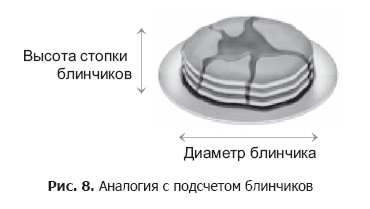
To count the pancakes, we separate one from the other along the vertical axis (that is, the height of the stack). However, if the stack is small, the CIM erroneously decides that the horizontal axis (diameter of pancakes) will be the best main component, due to the fact that in this measurement a greater scatter of values ​​can be found.

Interpretation of components. The main difficulty with CIM is that it is necessary to interpret the generated components, and sometimes you have to try very hard to explain why the variables must be combined in the chosen way.

Nevertheless, preliminary general information can help us out. In our example with products, it is the preliminary knowledge about their categories that helps us to combine food variables for the main components.

»More information about the book can be found atPublisher's website
» Table of contents
» Fragment

For Habrozhiteley 20% discount on the coupon - BigData