Transfer Learning: how to quickly train a neural network on your data
Machine learning becomes more accessible, there are more opportunities to apply this technology using “ready-made components”. For example, Transfer Learning allows you to use the experience gained in solving one task to solve another, similar problem. The neural network is first trained on a large amount of data, then on the target set.

In this article I will explain how to use the Transfer Learning method using the example of image recognition with food. I will talk about other machine learning tools at the workshop “Machine Learning and Neural Networks for Developers” .
If we are faced with the problem of image recognition, you can use a ready-made service. However, if you need to train a model on your own data set, you will have to do it yourself.
For such typical tasks as image classification, you can use a ready-made architecture (AlexNet, VGG, Inception, ResNet, etc.) and train the neural network on your data. Implementations of such networks using various frameworks already exist, so at this stage you can use one of them as a black box, without delving deeply into the principle of its operation.
However, deep neural networks are demanding large amounts of data for convergence learning. And often in our particular task there is not enough data to train all layers of the neural network well. Transfer Learning solves this problem.
Neural networks that are used for classification, as a rule, contain
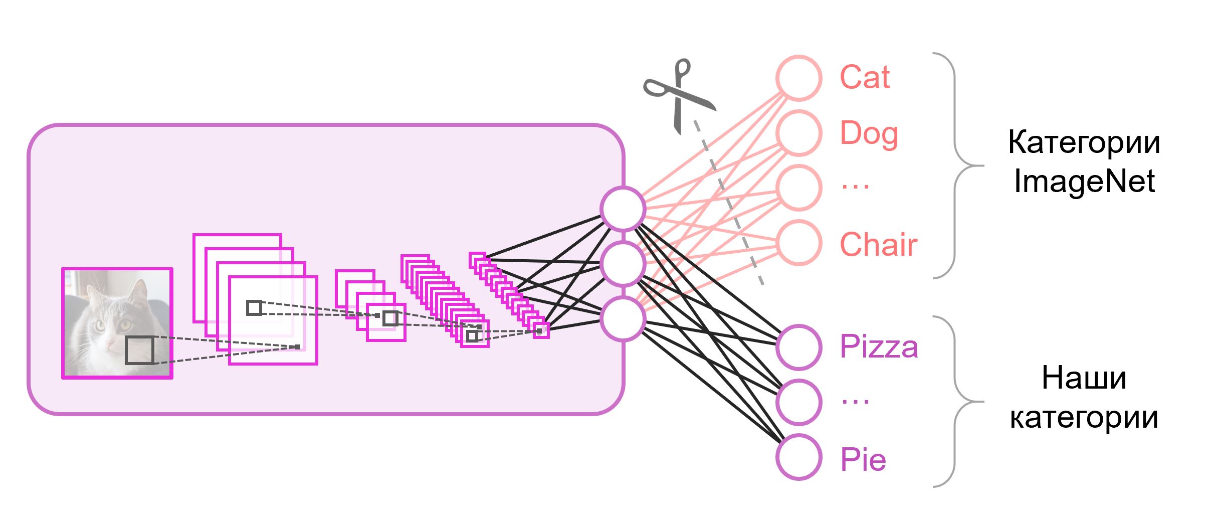
Often at the end of the classification networks a fully connected layer is used. Since we have replaced this layer, it will no longer be possible to use pre-trained weights for it. You have to train him from scratch, initializing his weights with random values. We load the weights for all other layers from the pre-trained snapshot.
There are various strategies for the additional training of the model. We will use the following: we will train the entire network from end to end ( end-to-end ), and we will not fix the pre-trained weights to give them a little correction and adjust to our data. This process is called fine tuning .
To solve the problem, we need the following components:
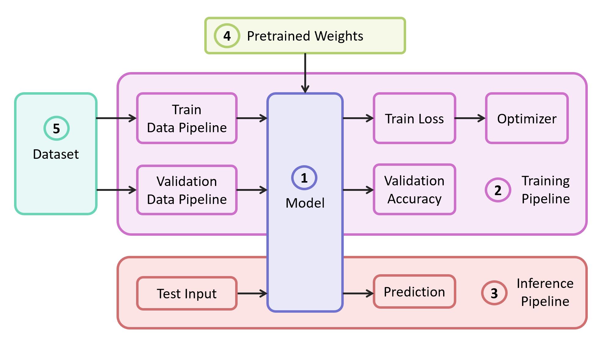
In our example, the components (1), (2) and (3) I will take from my own repository , which contains the most lightweight code - if you wish, you can easily figure it out. Our example will be implemented on the popular TensorFlow framework . The pre-learned weights (4), suitable for the chosen framework, can be found if they correspond to one of the classical architectures. As a dataset (5) for the demonstration I will take Food-101 .
As a model, we use the classic neural network VGG (more precisely, VGG19 ). Despite some shortcomings, this model shows a fairly high quality. In addition, it is easy to analyze. On TensorFlow Slim, the description of the model looks quite compact:
Weights for VGG19, trained on ImageNet and compatible with TensorFlow, will be downloaded from the repository to GitHub from the section Pre-trained Models .
As a training and validation sample, we will use the public dataset Food-101 , which contains more than 100 thousand images of food, divided into 101 categories.

Download and unpack datacat:
The data pipeline in our training is designed so that we need to parse the following from the dataset:
If yours, then the train and validation sets need to be broken independently. In Food-101 such a partition is already there, and this information is stored in a directory
All auxiliary functions responsible for data processing are moved to a separate file
The model learning code consists of the following steps:
The last layer of the graph is constructed with the number of neurons we need and is excluded from the list of parameters loaded from the pre-trained snapshot.
After starting the training, you can look at its progress using the TensorBoard utility, which comes bundled with TensorFlow and serves to visualize various metrics and other parameters.
At the end of training at TensorBoard, we see an almost perfect picture: a reduction in Train loss and an increase in Validation Accuracy

As a result, we get a saved snapshot in
Now let's test our model. For this:
All code, including resources for building and running the Docker container with all the necessary versions of libraries, is in this repository - at the time of reading the article, the code in the repository may have updates.
At the workshop “Machine Learning and Neural Networks for Developers” I will review other tasks of machine learning, and students will present their projects by the end of the intensive.
In this article I will explain how to use the Transfer Learning method using the example of image recognition with food. I will talk about other machine learning tools at the workshop “Machine Learning and Neural Networks for Developers” .
If we are faced with the problem of image recognition, you can use a ready-made service. However, if you need to train a model on your own data set, you will have to do it yourself.
For such typical tasks as image classification, you can use a ready-made architecture (AlexNet, VGG, Inception, ResNet, etc.) and train the neural network on your data. Implementations of such networks using various frameworks already exist, so at this stage you can use one of them as a black box, without delving deeply into the principle of its operation.
However, deep neural networks are demanding large amounts of data for convergence learning. And often in our particular task there is not enough data to train all layers of the neural network well. Transfer Learning solves this problem.
Transfer Learning for image classification
Neural networks that are used for classification, as a rule, contain
Noutput neurons in the last layer, where Nis the number of classes. Such an output vector is treated as a set of probabilities of belonging to a class. In our food image recognition task, the number of classes may differ from that in the original dataset. In this case, we will have to completely throw out this last layer and put a new one, with the necessary number of output neurons. Often at the end of the classification networks a fully connected layer is used. Since we have replaced this layer, it will no longer be possible to use pre-trained weights for it. You have to train him from scratch, initializing his weights with random values. We load the weights for all other layers from the pre-trained snapshot.
There are various strategies for the additional training of the model. We will use the following: we will train the entire network from end to end ( end-to-end ), and we will not fix the pre-trained weights to give them a little correction and adjust to our data. This process is called fine tuning .
Structural components
To solve the problem, we need the following components:
- Description of the neural network model
- Pipeline training
- Inference pipeline
- Pre-learned weights for this model
- Training and Validation Data
In our example, the components (1), (2) and (3) I will take from my own repository , which contains the most lightweight code - if you wish, you can easily figure it out. Our example will be implemented on the popular TensorFlow framework . The pre-learned weights (4), suitable for the chosen framework, can be found if they correspond to one of the classical architectures. As a dataset (5) for the demonstration I will take Food-101 .
Model
As a model, we use the classic neural network VGG (more precisely, VGG19 ). Despite some shortcomings, this model shows a fairly high quality. In addition, it is easy to analyze. On TensorFlow Slim, the description of the model looks quite compact:
import tensorflow as tf
import tensorflow.contrib.slim as slim
defvgg_19(inputs,
           num_classes,
           is_training,
           scope='vgg_19',
           weight_decay=0.0005):with slim.arg_scope([slim.conv2d],
                activation_fn=tf.nn.relu,
                weights_regularizer=slim.l2_regularizer(weight_decay),
                biases_initializer=tf.zeros_initializer(),
                padding='SAME'):
        with tf.variable_scope(scope, 'vgg_19', [inputs]):
            net = slim.repeat(inputs, 2, slim.conv2d, 64, [3, 3], scope='conv1')
            net = slim.max_pool2d(net, [2, 2], scope='pool1')
            net = slim.repeat(net, 2, slim.conv2d, 128, [3, 3], scope='conv2')
            net = slim.max_pool2d(net, [2, 2], scope='pool2')
            net = slim.repeat(net, 4, slim.conv2d, 256, [3, 3], scope='conv3')
            net = slim.max_pool2d(net, [2, 2], scope='pool3')
            net = slim.repeat(net, 4, slim.conv2d, 512, [3, 3], scope='conv4')
            net = slim.max_pool2d(net, [2, 2], scope='pool4')
            net = slim.repeat(net, 4, slim.conv2d, 512, [3, 3], scope='conv5')
            net = slim.max_pool2d(net, [2, 2], scope='pool5')
            # Use conv2d instead of fully_connected layers
            net = slim.conv2d(net, 4096, [7, 7], padding='VALID', scope='fc6')
            net = slim.dropout(net, 0.5, is_training=is_training, scope='drop6')
            net = slim.conv2d(net, 4096, [1, 1], scope='fc7')
            net = slim.dropout(net, 0.5, is_training=is_training, scope='drop7')
            net = slim.conv2d(net, num_classes, [1, 1], scope='fc8',
                activation_fn=None)
            net = tf.squeeze(net, [1, 2], name='fc8/squeezed')
    return net
Weights for VGG19, trained on ImageNet and compatible with TensorFlow, will be downloaded from the repository to GitHub from the section Pre-trained Models .
mkdir data && cd data
wget http://download.tensorflow.org/models/vgg_19_2016_08_28.tar.gz
tar -xzf vgg_19_2016_08_28.tar.gz
Dataset
As a training and validation sample, we will use the public dataset Food-101 , which contains more than 100 thousand images of food, divided into 101 categories.
Download and unpack datacat:
cd data
wget http://data.vision.ee.ethz.ch/cvl/food-101.tar.gz
tar -xzf food-101.tar.gz
The data pipeline in our training is designed so that we need to parse the following from the dataset:
- List of classes (categories)
- Training kit: a list of paths to pictures and a list of correct answers
- Validation set: list of paths to pictures and list of correct answers
If yours, then the train and validation sets need to be broken independently. In Food-101 such a partition is already there, and this information is stored in a directory
meta.DATASET_ROOT = 'data/food-101/'
train_data, val_data, classes = data.food101(DATASET_ROOT)
num_classes = len(classes)
All auxiliary functions responsible for data processing are moved to a separate file
data.py:data.py
from os.path import join as opj
import tensorflow as tf
defparse_ds_subset(img_root, list_fpath, classes):'''
    Parse a meta file with image paths and labels
    -> img_root: path to the root of image folders
    -> list_fpath: path to the file with the list (e.g. train.txt)
    -> classes: list of class names
    <- (list_of_img_paths, integer_labels)
    '''
    fpaths = []
    labels = []
    with open(list_fpath, 'r') as f:
        for line in f:
            class_name, image_id = line.strip().split('/')
            fpaths.append(opj(img_root, class_name, image_id+'.jpg'))
            labels.append(classes.index(class_name))
    return fpaths, labels
deffood101(dataset_root):'''
    Get lists of train and validation examples for Food-101 dataset
    -> dataset_root: root of the Food-101 dataset
    <- ((train_fpaths, train_labels), (val_fpaths, val_labels), classes)
    '''
    img_root = opj(dataset_root, 'images')
    train_list_fpath = opj(dataset_root, 'meta', 'train.txt')
    test_list_fpath = opj(dataset_root, 'meta', 'test.txt')
    classes_list_fpath = opj(dataset_root, 'meta', 'classes.txt')
    with open(classes_list_fpath, 'r') as f:
        classes = [line.strip() for line in f]
    train_data = parse_ds_subset(img_root, train_list_fpath, classes)
    val_data = parse_ds_subset(img_root, test_list_fpath, classes)
    return train_data, val_data, classes
defimread_and_crop(fpath, inp_size, margin=0, random_crop=False):'''
    Construct TF graph for image preparation:
    Read the file, crop and resize
    -> fpath: path to the JPEG image file (TF node)
    -> inp_size: size of the network input (e.g. 224)
    -> margin: cropping margin
    -> random_crop: perform random crop or central crop
    <- prepared image (TF node)
    '''
    data = tf.read_file(fpath)
    img = tf.image.decode_jpeg(data, channels=3)
    img = tf.image.convert_image_dtype(img, dtype=tf.float32)
    shape = tf.shape(img)
    crop_size = tf.minimum(shape[0], shape[1]) - 2 * margin
    if random_crop:
        img = tf.random_crop(img, (crop_size, crop_size, 3))
    else: # central crop
        ho = (shape[0] - crop_size) // 2
        wo = (shape[0] - crop_size) // 2
        img = img[ho:ho+crop_size, wo:wo+crop_size, :]
    img = tf.image.resize_images(img, (inp_size, inp_size),
        method=tf.image.ResizeMethod.AREA)
    return img
deftrain_dataset(data, batch_size, epochs, inp_size, margin):'''
    Prepare training data pipeline
    -> data: (list_of_img_paths, integer_labels)
    -> batch_size: training batch size
    -> epochs: number of training epochs
    -> inp_size: size of the network input (e.g. 224)
    -> margin: cropping margin
    <- (dataset, number_of_train_iterations)
    '''
    num_examples = len(data[0])
    iters = (epochs * num_examples) // batch_size
    deffpath_to_image(fpath, label):
        img = imread_and_crop(fpath, inp_size, margin, random_crop=True)
        return img, label
    dataset = tf.data.Dataset.from_tensor_slices(data)
    dataset = dataset.shuffle(buffer_size=num_examples)
    dataset = dataset.map(fpath_to_image)
    dataset = dataset.repeat(epochs)
    dataset = dataset.batch(batch_size, drop_remainder=True)
    return dataset, iters
defval_dataset(data, batch_size, inp_size):'''
    Prepare validation data pipeline
    -> data: (list_of_img_paths, integer_labels)
    -> batch_size: validation batch size
    -> inp_size: size of the network input (e.g. 224)
    <- (dataset, number_of_val_iterations)
    '''
    num_examples = len(data[0])
    iters = num_examples // batch_size
    deffpath_to_image(fpath, label):
        img = imread_and_crop(fpath, inp_size, 0, random_crop=False)
        return img, label
    dataset = tf.data.Dataset.from_tensor_slices(data)
    dataset = dataset.map(fpath_to_image)
    dataset = dataset.batch(batch_size, drop_remainder=True)
    return dataset, iters
Model training
The model learning code consists of the following steps:
- Building the train / validation data pipelines
- Building train / validation graphs (networks)
- Building the entropy loss over the train graph
- The code needed to calculate the prediction accuracy on a validation sample during training
- Logic loading pre-trained scales from snapshot
- Creating different structures for learning
- Directly the learning cycle itself (iterative optimization)
The last layer of the graph is constructed with the number of neurons we need and is excluded from the list of parameters loaded from the pre-trained snapshot.
Model Learning Code
import numpy as np
import tensorflow as tf
import tensorflow.contrib.slim as slim
tf.logging.set_verbosity(tf.logging.INFO)
import model
import data
##############################################################  Settings###########################################################
INPUT_SIZE = 224
RANDOM_CROP_MARGIN = 10
TRAIN_EPOCHS = 20
TRAIN_BATCH_SIZE = 64
VAL_BATCH_SIZE = 128
LR_START = 0.001
LR_END = LR_START / 1e4
MOMENTUM = 0.9
VGG_PRETRAINED_CKPT = 'data/vgg_19.ckpt'
CHECKPOINT_DIR = 'checkpoints/vgg19_food'
LOG_LOSS_EVERY = 10
CALC_ACC_EVERY = 500##############################################################  Build training and validation data pipelines###########################################################
train_ds, train_iters = data.train_dataset(train_data,
    TRAIN_BATCH_SIZE, TRAIN_EPOCHS, INPUT_SIZE, RANDOM_CROP_MARGIN)
train_ds_iterator = train_ds.make_one_shot_iterator()
train_x, train_y = train_ds_iterator.get_next()
val_ds, val_iters = data.val_dataset(val_data,
    VAL_BATCH_SIZE, INPUT_SIZE)
val_ds_iterator = val_ds.make_initializable_iterator()
val_x, val_y = val_ds_iterator.get_next()
##############################################################  Construct training and validation graphs###########################################################with tf.variable_scope('', reuse=tf.AUTO_REUSE):
    train_logits = model.vgg_19(train_x, num_classes, is_training=True)
    val_logits = model.vgg_19(val_x, num_classes, is_training=False)
##############################################################  Construct training loss###########################################################
loss = tf.losses.sparse_softmax_cross_entropy(
    labels=train_y, logits=train_logits)
tf.summary.scalar('loss', loss)
##############################################################  Construct validation accuracy###  and related functions###########################################################defcalc_accuracy(sess, val_logits, val_y, val_iters):
    acc_total = 0.0
    acc_denom = 0for i in range(val_iters):
        logits, y = sess.run((val_logits, val_y))
        y_pred = np.argmax(logits, axis=1)
        correct = np.count_nonzero(y == y_pred)
        acc_denom += y_pred.shape[0]
        acc_total += float(correct)
        tf.logging.info('Validating batch [{} / {}] correct = {}'.format(
            i, val_iters, correct))
    acc_total /= acc_denom
    return acc_total
defaccuracy_summary(sess, acc_value, iteration):
    acc_summary = tf.Summary()
    acc_summary.value.add(tag="accuracy", simple_value=acc_value)
    sess._hooks[1]._summary_writer.add_summary(acc_summary, iteration)
##############################################################  Define set of VGG variables to restore###  Create the Restorer###  Define init callback (used by monitored session)###########################################################
vars_to_restore = tf.contrib.framework.get_variables_to_restore(
    exclude=['vgg_19/fc8'])
vgg_restorer = tf.train.Saver(vars_to_restore)
definit_fn(scaffold, sess):
    vgg_restorer.restore(sess, VGG_PRETRAINED_CKPT)
##############################################################  Create various training structures###########################################################
global_step = tf.train.get_or_create_global_step()
lr = tf.train.polynomial_decay(LR_START, global_step, train_iters, LR_END)
tf.summary.scalar('learning_rate', lr)
optimizer = tf.train.MomentumOptimizer(learning_rate=lr, momentum=MOMENTUM)
training_op = slim.learning.create_train_op(
    loss, optimizer, global_step=global_step)
scaffold = tf.train.Scaffold(init_fn=init_fn)
##############################################################  Create monitored session###  Run training loop###########################################################with tf.train.MonitoredTrainingSession(checkpoint_dir=CHECKPOINT_DIR,
                                       save_checkpoint_secs=600,
                                       save_summaries_steps=30,
                                       scaffold=scaffold) as sess:
    start_iter = sess.run(global_step)
    for iteration in range(start_iter, train_iters):
        # Gradient Descent
        loss_value = sess.run(training_op)
        # Loss loggingif iteration % LOG_LOSS_EVERY == 0:
            tf.logging.info('[{} / {}] Loss = {}'.format(
                iteration, train_iters, loss_value))
        # Accuracy loggingif iteration % CALC_ACC_EVERY == 0:
            sess.run(val_ds_iterator.initializer)
            acc_value = calc_accuracy(sess, val_logits, val_y, val_iters)
            accuracy_summary(sess, acc_value, iteration)
            tf.logging.info('[{} / {}] Validation accuracy = {}'.format(
                iteration, train_iters, acc_value))
After starting the training, you can look at its progress using the TensorBoard utility, which comes bundled with TensorFlow and serves to visualize various metrics and other parameters.
tensorboard --logdir checkpoints/
At the end of training at TensorBoard, we see an almost perfect picture: a reduction in Train loss and an increase in Validation Accuracy
As a result, we get a saved snapshot in
checkpoints/vgg19_food, which we will use during our model testing ( inference ).Model testing
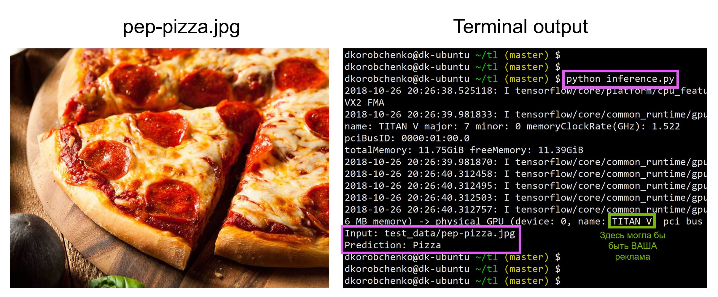
Now let's test our model. For this:
- We construct a new graph designed specifically for inference (
is_training=False) - Load the trained weights from the snapshot
- Load and pre-process the input test image.
- Let's drive the image through the neural network and get the prediction
inference.py
import sys
import numpy as np
import imageio
from skimage.transform import resize
import tensorflow as tf
import model
##############################################################  Settings###########################################################
CLASSES_FPATH = 'data/food-101/meta/labels.txt'
INP_SIZE = 224# Input will be cropped and resized
CHECKPOINT_DIR = 'checkpoints/vgg19_food'
IMG_FPATH = 'data/food-101/images/bruschetta/3564471.jpg'##############################################################  Get all class names###########################################################with open(CLASSES_FPATH, 'r') as f:
    classes = [line.strip() for line in f]
num_classes = len(classes)
##############################################################  Construct inference graph###########################################################
x = tf.placeholder(tf.float32, (1, INP_SIZE, INP_SIZE, 3), name='inputs')
logits = model.vgg_19(x, num_classes, is_training=False)
##############################################################  Create TF session and restore from a snapshot###########################################################
sess = tf.Session()
snapshot_fpath = tf.train.latest_checkpoint(CHECKPOINT_DIR)
restorer = tf.train.Saver()
restorer.restore(sess, snapshot_fpath)
##############################################################  Load and prepare input image###########################################################defcrop_and_resize(img, input_size):
    crop_size = min(img.shape[0], img.shape[1])
    ho = (img.shape[0] - crop_size) // 2
    wo = (img.shape[0] - crop_size) // 2
    img = img[ho:ho+crop_size, wo:wo+crop_size, :]
    img = resize(img, (input_size, input_size),
        order=3, mode='reflect', anti_aliasing=True, preserve_range=True)
    return img
img = imageio.imread(IMG_FPATH)
img = img.astype(np.float32)
img = crop_and_resize(img, INP_SIZE)
img = img[None, ...]
##############################################################  Run inference###########################################################
out = sess.run(logits, feed_dict={x:img})
pred_class = classes[np.argmax(out)]
print('Input: {}'.format(IMG_FPATH))
print('Prediction: {}'.format(pred_class))
All code, including resources for building and running the Docker container with all the necessary versions of libraries, is in this repository - at the time of reading the article, the code in the repository may have updates.
At the workshop “Machine Learning and Neural Networks for Developers” I will review other tasks of machine learning, and students will present their projects by the end of the intensive.