Simple fuzzy logic blinded "from what it was" for a gas turbine engine
- Tutorial
By chance, in my hands was “all regime component-wise model of an aircraft engine” from a solid developer of the Central Institute of Aviation Motors (CIAM), and of course I wanted to try on it all these regulators, which are considered on simple or simplified models of the unit. By my education, I am a designer of nuclear reactors, and about an aircraft engine, I only know that it can fall onto the protective shell of the reactor along with the aircraft and it must withstand. Before we torture a real model, we will practice on cats, before switching to the turbojet, we will torture a simple gas turbine model.
In this article we will create a regulator model based on the standard library of structural modeling (without using a ready-made library of fuzzy regulation blocks).
The model of the gas turbine engine from the textbook V.I. Guest “Fuzzy controllers in automatic control systems”
Let us make a comparison with PID and traffic regulations regulators.
And as an illustrative demonstration in the next article, we will regulate not a simplified, but a real model of a real engine, which is used by CIAM. Baranov.
Formulation of the problem
The difference between a gas turbine engine (GTE) and a turbojet (TRD) is that in a GTE all energy is removed through the shaft. In TRD, energy is released in the form of a jet stream.
Gas turbine engines (GTE) are widely used in the gas and aviation industry, where they are the basis of gas pumping units and aircraft power plants, in drives of industrial electric turbogenerators of peak and mobile power plants, in ship power plants and at other industrial facilities where the development of large unit capacities (from 1 to 25 MW) in one unit with its minimum mass and dimensions.
Gas turbine engines are presented with a set of requirements related to their reliability, energy efficiency, safety and environmental friendliness during operation. Along with these requirements, the requirements for the quality of transients associated with the launch of the unit, a sharp change in the selected load (power) are relevant. In many respects, the satisfaction of these requirements lies with the automatic control system (ACS) of the CCD.
A typical gas turbine engine, which is used in industry, is a turboshaft engine, the scheme of which is shown in Figure 1.
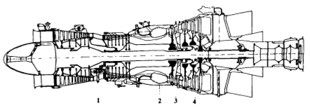
Figure 1. Diagram of a typical industrial gas turbine engine:
1-compressor; 2 - combustion chamber; 3 - compressor turbine; 4 - power turbine.
The engine is a rotary machine in which air is compressed in compressor 1, combustion process of fuel supplied to air is carried out in combustion chamber 2, and part of the energy in the turbine of compressor 3 is extracted from hot gases, consumed to drive compressor 1, in gas turbine 4 expanding to create power taken from the engine by the consumer.
In the vast majority of gas turbine engines, the rotor speed is a controllable value. As a control factor in the ACS, the rotor speed n uses the fuel consumption Gт into the combustion chamber. At different operating modes and under different external conditions, the parameters of the engine change significantly.
Consider a gas turbine engine (GTE) as a non-stationary control object for which the rotor speed is n controlled variable, and the fuel consumption G T is a control action. Linearizing depending turbine torque - M T and the time the compressor - M K , from the rotor speed and without considering the influence of heat and mass capacity for a particular engine operating mode write transfer motor function as follows:
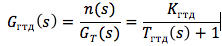
where the gain and time constant are defined as:
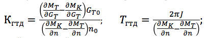
moreover, the input and output signals are recorded in relative dimensionless deviations from the steady state (n = Δn / n 0 ; G T = ΔG / G TO , where the basic values of the parameters are selected for a specific mode of engine operation, for example, nominal or maximum). In different operating modes and under different external conditions, the gain and the time constant of the engine vary significantly, therefore, for each mode it is necessary to determine its own values of K GTE and T GTE .
Note that the transfer function G GTD (s) for a non-stationary control object, such as a gas turbine engine, was obtained by the method of “frozen” coefficients, provided that the object parameters are sufficiently slow.
The block diagram of the analog electromechanical system of automatic control of the rotor speed of the engine is shown in Figure 2.
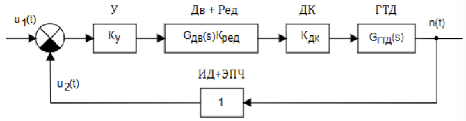
Figure 2. Block diagram of the analog CCD GTE
The frequency of rotation is given by the voltage u 1 (t) and is changed by a pulse ID sensor, the frequency of the output signal of which is determined by the expression:
f = kmn, where n is the number of engine revolutions, m is the number of gear teeth, k is the transmission coefficient. The alternating voltage taken from the ID output by means of an electronic frequency converter (EPC) is converted into a signal u2 (t), the value of which is proportional to the engine speed - n. The voltage u2 (t) is compared with the reference voltage and the error signal after the amplifier Y is fed to a two-phase asynchronous motor Dv, which through the Red reducer regulates the throttle valve of the DC, changing the consumption of fuel entering the gas turbine engine. A pulse sensor together with an electronic frequency converter can be described by a proportional link with a transfer function equal to one. In this case, the system itself has a single feedback.
Considering the serial connection of an amplifier, an induction motor, a throttle valve, a gas turbine unit and a frequency sensor with an electronic frequency converter as a common control object, and using a digital fuzzy controller, the entire block diagram from Figure 2 can be reduced to the block diagram in Figure 3. All of this the transfer functions of links are reduced to a common transfer function G 0 (s).
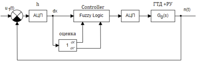
Figure 3. The structure of the control system with a fuzzy regulator.
The total transfer function G0 (s) can be written as:
G 0 (s) = K Y G DV (s) K RED K DK G GTE (s) = α [s (s + a) (s + b)] -1 , where
α = abK U K DV K KED To DK K GTE ,
a = 1 / T DV ,
b = 1 / T GTE
For example, we assume that the dependencies of the transfer function on the operation time take the following values:
T GTE (t) = 0.9849 - 0.1188 × t + 0.0063 × t 2 - 0.00012 × t 3 ;
α (t) = 16.5475 - 4.4469 × t + 0.4843 × t 2 - 0.02315 × t 3 + 0.0004 × t 4 ;
T DV = 0,35 c.
In the study of the control system, we assume that the given function of changing the rotor speed of a gas turbine engine is given by the input voltage u (t)
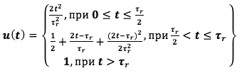
where τ r is the engine acceleration time. Accept τ r = 6 seconds.
Creating a dynamic model
A simplified model of the engine is shown in Figure 4. In this model, we use the variable parameters of the typical blocks, which vary in the process of modeling the dependencies given above.
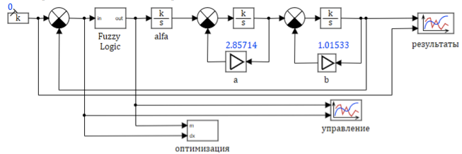
Figure 4. Block diagram of the GTE model
The coefficients alfa, a, b amplifiers are calculated using a scripting language, the program text below:
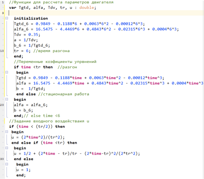
Figure 5. Script for calculating model parameters.
Fuzzy Logic Control Regulator
The control knob takes the mismatch between the set value and the value obtained from the model and must calculate the control action.
Let's try to assemble a regulator based on fuzzy logic, using only standard mathematically blocks of structural modeling, without using a specialized library.
A description of the principles of control based on fuzzy logic can be found in the previous article on Habré, or in the description of creating a specialized library of blocks here (cautiously, profanity).
Any controller based on fuzzy logic performs the following sequence of transformations:
- Phasification of input variables. The value of the variable is replaced by a set of terms.
- Activation of the conclusions of the rules of fuzzy logic.
- Accumulation of conclusions for each linguistic variable.
- De-phasing of output variables.
To control the engine, we will use three continuous variables that are calculated on the basis of a single signal:
- deviation;
- derivative deviation (rate of change deviation);
- the second derivative of the deviation (acceleration of changes in deviations).
The calculation scheme is presented in Figure 6:
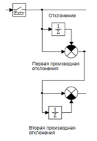
Figure 6. Calculations of the first and second derivatives of the deviation.
The extrapolator block quantizes the signal entering the controller with a period of 0.01 sec. The first and second derivatives are calculated using difference formulas:
 Where:
u (t) is the current deviation value at time t;
u (t-Δt) is the deviation value at time t - Δt;
u '(t) is the current value of the derivative of the deviation at time t;
u '(t-Δt) is the value of the derivative of the deviation at time t - Δt;
u '' (t) is the current value of the second derivative of the deviation at time t;
u "(t-Δt) is the value of the second derivative of the deviation at time t - Δt;
Δt is the quantization period.
The division by Δt is performed in the comparison unit.
As a result of this block, three linguistic variables are created: deviation, first deviation variable, second deviation variable.
To solve the fuzzy control problem, we will use only two terms for each linguistic variable.
Deviation - less, more;
The first derivative of the deviation decreases, increases;
The second derivative of the deviation is slowing, accelerating.
To calculate the value of the membership function μ for each term, we use a linear function with saturation. This function for the term is greater than 0 when the input value is minimum and 1 when the input value is maximum. For a term less, this function takes the value 1 when the variable is equal to the minimum, and 0 when the variable is maximum. (see fig. 7)
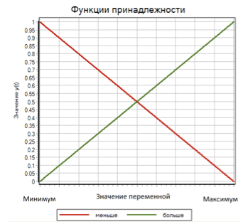
Figure 7. Membership functions for terms less and more.
Thus, for each of the three input variables (deviation, 1st derivative of deviation, 2nd derivative of deviation) two terms appear more and less, the value of the membership functions μ i which vary linearly from 0 to 1 depending on the value of the input variable.
As an output linguistic variable, we use an output effect that also has only two terms decreasing and increasing.
From the diagram of the model in fig. 4 it is obvious that if the deviation is less than 0, then the value is greater than the specified one and must be reduced. If the deviation is greater than 0, then the function is less than the specified one and must be increased.
The logical rules for two terms will look like this:
- If less and decreases and slows down => decrease.
- If more and increases and accelerate => increase.
To activate the fuzzy inference rules, we use the function minimum for the fuzzy operator and. The value of the membership functions for the terms of the output function are calculated by the formulas:
μ decrease = MIN (μ less , μ decreases , μ slows down )
μ increase = MIN (μ more , μ increases , μ accelerates )
To ensure that terms are converted to specific values of exposure (accumulation and denazification), we use the Tsukamoto algorithm (Tsukamoto) as the center of gravity of the points.
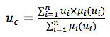 where,
u c - the resulting function;
u i - the value of the function for the term i;
μ i - the value of the membership function for terms for the function.
In our case, the resulting function for two terms is calculated by the formula: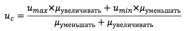
The general scheme of the fuzzy inference algorithm is presented in Figure 8:
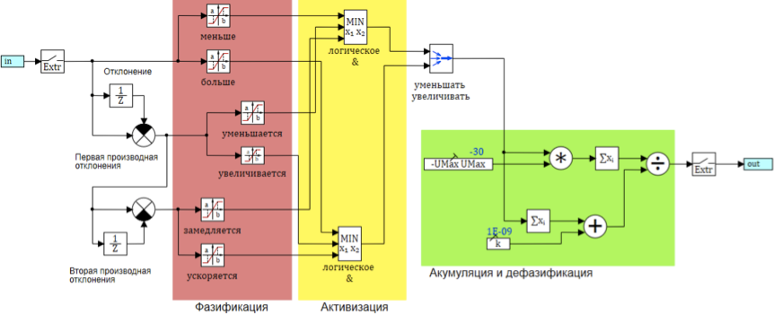
Figure 8. Fuzzy inference algorithm
In order for this algorithm to work, we must specify the minimum and maximum values for 6 terms of three linguistic variables (deviation, 1st derivative of deviation, 2nd derivative of deviation). To reduce the calculations, we assume that the deviation is symmetric about zero. Then we only need to find 3 absolute values, one for each variable.
deltMax - the maximum deviation. Sets the values of terms less, greater (-deltMax, deltaMax);
divMax is the maximum derivative of the deviation. Sets the values of terms decreases, increases (-divMax, divMax);
div2Max - maximum second derivative. Sets the values of terms slowed, accelerated (-div2Max, div2Max).
The maximum and minimum effects of umin and umax are determined by the design features and in this example are assumed to be +30 and -30.
Adjustment controller optimization.
For the selection of coefficients, we use the same optimization scheme that we used in previous experiments with fuzzy logic.
As optimization criteria, we take the standard deviation of not more than 0.001 and the number of switches in the control unit no more than 25. For switching, we take the change of the sign of the control action.
The circuit of the regulator tuning block is presented in fig. 9.
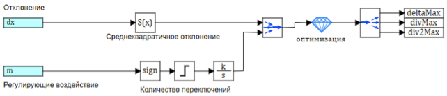
Figure 9. Configuring Fuzzy Output Parameters.
As a result of the block operation, the following parameters were obtained
deltMax = 0.00746;
divMax = 0.2657;
div2Max = 25.13;
The results of the transition process are shown in Figure 10.
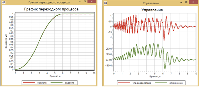
Figure 10. Transient and motor control using fuzzy logic.
The maximum deviation of turns from the given after optimization was 2.5 × 10 -3 . That, in principle, is not bad, however, in the book of V.I. The guest deviations in the model after adjustments were two orders of magnitude smaller: the maximum was 5 × 10 -5 .
For comparison, we present the results of the PID controller Fig.11 and the traffic regulations Fig.12 for the same model of a simplified engine. The parameters of these regulators were also selected by the optimization method.
As a result, a larger deviation was obtained for the PID controller than for a controller based on fuzzy logic - about 6 × 10 -3 , and for the PDA controller that uses the second derivative, the deviation turned out to be about 3 × 10 -3 (see 13). At the same time, in all the graphs it can be seen that with a change in a given effect (changes in the sections of 3 s, 6 s) the quality of regulation changes.
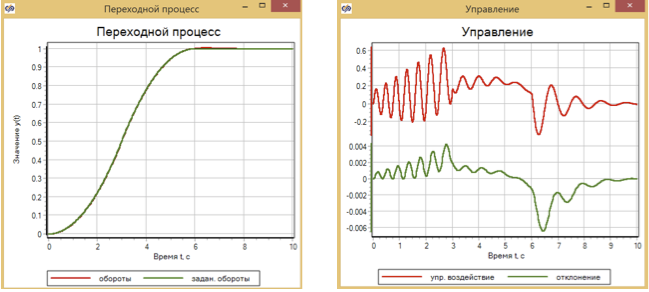
Figure 11. Transient and motor control using the PID controller.
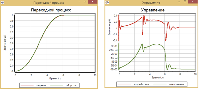
Figure 12. Transient and engine control using the PDA controller.
To start the engine, the transition function is used in the form of a smooth change in revolutions. We have also adjusted the regulators by optimizing for optimal control exactly according to this law. Let's try to apply a stepped effect and see how the regulators, initially optimized for a smooth transition process, can handle.
As an impact, we use a step from 0 to 1 for 3 seconds of the process.
The results of the experiment are presented in Figures 13 - 15.
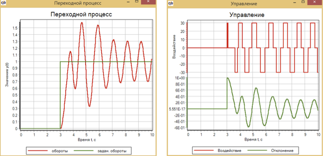
Figure 13. Transient process and control with step control with a fuzzy logic controller.
It can be seen that the regulator, which is configured for smooth acceleration of the engine, does not cope with the control, and the system goes into self-oscillation mode.
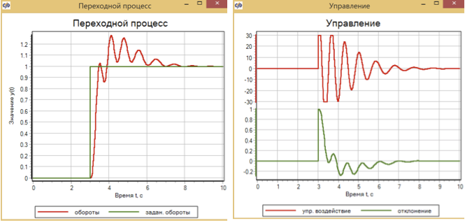
Figure 14. Transient and step control with a PID regulator.
The PID controller, which is set to a smooth process, with a step effect provides a transition at a specified time, but this causes an overshoot by 30% and an oscillatory process within 4 seconds.
A traffic controller that is configured for smooth control, with a step effect, provides a smooth transition without overshoot (Fig. 14)
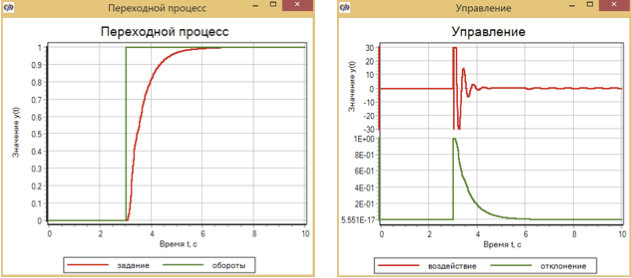
Figure 15. Transient process and control with step control with a traffic controller.
findings
The above numerical experiments showed that the controller based on fuzzy logic provides more precise control of the speed of a simple engine model with a smooth change of the setpoint than the PID and traffic control.
However, such a setting, as it turned out, does not guarantee the stability of the regulator under step action.
At the same time, for a simplified model of the engine, the regulator based on fuzzy logic turned out to be worse in the case of stepwise action than the PID or traffic controller.
Link to the archive with projects from the article for self-study