Monte Carlo simulation in Mathcad Express
- Tutorial
On Habré many articles are devoted to Monte Carlo algorithms, for example, this one, yesterday . Both the main idea and the implementation of the methods are very simple, but the lack of suitable modeling tools at hand can serve as a small obstacle. For those readers for whom the problem is relevant, I advise you to use the free mathematical editor Mathcad Express, about which I write in my blog .
Mathcad Express is the “light” version of the well-known PTC Mathcad Prime package, in which most of the functionality is turned off. Nevertheless, pseudo-random number sensors remain available, which allows you to implement (quite quickly and clearly) various statistical models based on Monte Carlo algorithms. I must say right away that some solutions will not be the best, from the point of view of users of the commercial version of Mathcad Prime, however, they are guaranteed not to lead us beyond the functionality of the free Mathcad Express.
Let me remind you that Monte Carlo algorithms are the general name of a group of numerical methods based on the programmatic creation of a certain sequence of pseudorandom numbers simulating a particular effect, for example, a sequence of equipment failures. Having received a large number of realizations of a random process, we can hope that its probabilistic characteristics will coincide with similar values of the problem of the "real world" being solved. A file with further calculations in the Mathcad and XPS formats lies here .
Mathcad Express has a number of pseudo-random number generators available that create pseudo-random data samples with different distribution laws. To create a vector from N pseudorandom numbers, you need only one line of a Mathcad document. For example, to generate N = 5 pseudo-random numbers with a normal distribution (zero mean and unit variance), you can do this: It

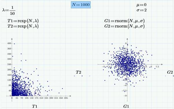
is convenient to visualize random number vectors on graphs as follows: one sample (i.e., components of one of the random vectors T1 ) along the abscissa axis, and another sample (another random vector T2 ) - along the ordinate axis. The following figure shows plots of pseudo-random number pairs for the exponential (left) and normal (right) distribution. Distribution parameters are set in the formulas above the graphs.
The following figure shows similar pairs of pseudorandom numbers G1 and G3 with normal distribution and different dispersion (graph on the left) and the method of generating correlated pseudorandom numbers G1 and G4 (graph on the right).

Generally speaking, quite a few pseudo-random number sensors are available in Mathcad Express:
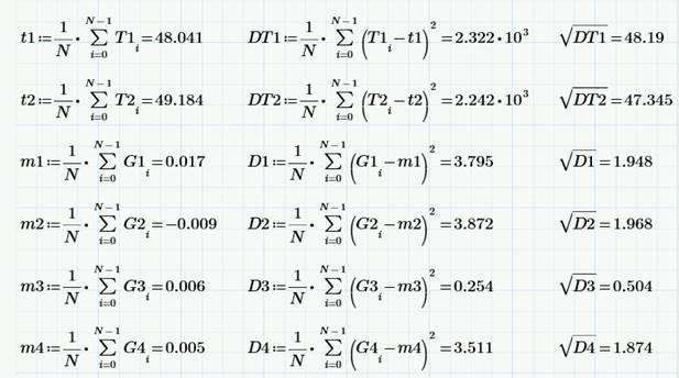
Using the simplest statistics formulas, one can calculate sample estimates of mean values, variances, and standard deviations:
Similarly, one can estimate the sample correlation coefficient:

An example of modeling the conversion of site visitors using correlated pseudorandom numbers I gave in an article on correlation and regression .
Here is a simple recipe for building a histogram chart. In the commercial version of Mathcad Prime, the preparation of data for a histogram is reduced to the use of one built-in function:
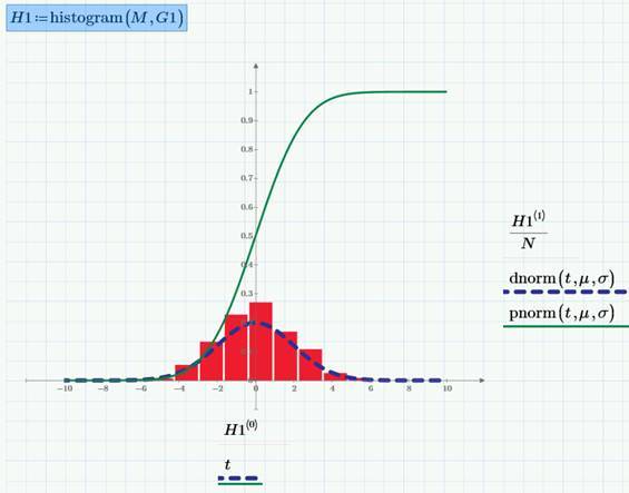
(By the way, for the listed types of distributions, there are also built-in functions for both probability density and distribution functions, as shown in the example of a Gaussian pseudo-random sampling). To plot a histogram in Mathcad Express, you must manually divide the interval (a, b) into which the data falls into M intervals and perform the simple mathematical operations available in Mathcad Express (which, if the reader is interested, he will find in the document with calculations ).

As an example, we use pseudo-random data with an exponential distribution (one of the practical applications of which is described in a previous article ).
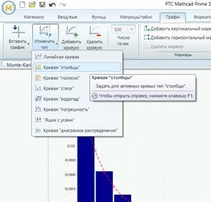
In conclusion, we note that for the histogram you should choose the appropriate type of graph:
To summarize: using the free mathematical package RTS Mathcad Express, you can quite easily implement Monte Carlo models in the usual mathematical notation and without resorting to programming. I also hope that I will be able to tell about other applications of Mathcad in data analysis in the following articles.
Mathcad Express is the “light” version of the well-known PTC Mathcad Prime package, in which most of the functionality is turned off. Nevertheless, pseudo-random number sensors remain available, which allows you to implement (quite quickly and clearly) various statistical models based on Monte Carlo algorithms. I must say right away that some solutions will not be the best, from the point of view of users of the commercial version of Mathcad Prime, however, they are guaranteed not to lead us beyond the functionality of the free Mathcad Express.
Let me remind you that Monte Carlo algorithms are the general name of a group of numerical methods based on the programmatic creation of a certain sequence of pseudorandom numbers simulating a particular effect, for example, a sequence of equipment failures. Having received a large number of realizations of a random process, we can hope that its probabilistic characteristics will coincide with similar values of the problem of the "real world" being solved. A file with further calculations in the Mathcad and XPS formats lies here .
Part 1. How to generate a selection of pseudo random numbers
Mathcad Express has a number of pseudo-random number generators available that create pseudo-random data samples with different distribution laws. To create a vector from N pseudorandom numbers, you need only one line of a Mathcad document. For example, to generate N = 5 pseudo-random numbers with a normal distribution (zero mean and unit variance), you can do this: It
is convenient to visualize random number vectors on graphs as follows: one sample (i.e., components of one of the random vectors T1 ) along the abscissa axis, and another sample (another random vector T2 ) - along the ordinate axis. The following figure shows plots of pseudo-random number pairs for the exponential (left) and normal (right) distribution. Distribution parameters are set in the formulas above the graphs.
The following figure shows similar pairs of pseudorandom numbers G1 and G3 with normal distribution and different dispersion (graph on the left) and the method of generating correlated pseudorandom numbers G1 and G4 (graph on the right).
Generally speaking, quite a few pseudo-random number sensors are available in Mathcad Express:
- rnd (x) is the uniform distribution on the interval (0, x).
- rbeta (x, s1, s2) - beta distribution (s1, s2> 0 - parameters, 0
- rbinom (k, n, p) - binomial distribution (n - integer parameter, 0
- rcauchy (x, l, s) is the Cauchy distribution (l is the expansion parameter, s> 0 is the scale parameter).
- rexp (x, r) is the exponential distribution (r> 0 is the exponent).
- rF (x, d1, d2) is the Fisher distribution (d1, d2> 0 are the degrees of freedom).
- rgamma (x, s) is the gamma distribution (s> 0 is the shape parameter).
- rgeom (k, p) - geometric distribution (0
- rhypergeom (k, a, b, n) - hypergeometric distribution (a, b, n - integer parameters).
- rlnorm (x, m, s) is the lognormal distribution (m is the natural logarithm of the mathematical expectation, s> 0 is the natural logarithm of the standard deviation).
- rlogis (x, l, s) - logistic distribution (l - mathematical expectation, s> 0 - scale parameter).
- rnbinom (k, n, p) - negative binomial distribution (n> 0 - integer parameter, 0
- rnorm (x, m, s) is the normal distribution (m is the average value, s> 0 is the standard deviation).
- rpois (k, p) is the Poisson distribution (p> 0 is the parameter).
- rt (x, d) is the student distribution (d> 0 is the number of degrees of freedom).
- runif (x, a, b) - uniform distribution (a
- rweibull (x, s) is the Weibull distribution (s> 0 is the parameter).
Part 2. How to perform statistical calculations
Using the simplest statistics formulas, one can calculate sample estimates of mean values, variances, and standard deviations:
Similarly, one can estimate the sample correlation coefficient:
An example of modeling the conversion of site visitors using correlated pseudorandom numbers I gave in an article on correlation and regression .
Part 3. How to build a histogram
Here is a simple recipe for building a histogram chart. In the commercial version of Mathcad Prime, the preparation of data for a histogram is reduced to the use of one built-in function:
(By the way, for the listed types of distributions, there are also built-in functions for both probability density and distribution functions, as shown in the example of a Gaussian pseudo-random sampling). To plot a histogram in Mathcad Express, you must manually divide the interval (a, b) into which the data falls into M intervals and perform the simple mathematical operations available in Mathcad Express (which, if the reader is interested, he will find in the document with calculations ).
As an example, we use pseudo-random data with an exponential distribution (one of the practical applications of which is described in a previous article ).
In conclusion, we note that for the histogram you should choose the appropriate type of graph:
To summarize: using the free mathematical package RTS Mathcad Express, you can quite easily implement Monte Carlo models in the usual mathematical notation and without resorting to programming. I also hope that I will be able to tell about other applications of Mathcad in data analysis in the following articles.