Buying an optimal apartment with R
Many people are faced with the issue of buying or selling real estate, and an important criterion here is not to buy more expensive or not to sell cheaper relative to other, comparable options. The simplest way is a comparative one, focusing on the average price of a meter in a particular place and expertly adding or lowering percentages of the cost for the advantages and disadvantages of a particular apartment. But this approach is time-consuming, inaccurate and will not allow to take into account all the variety of differences of apartments from each other. Therefore, I decided to automate the process of selecting real estate using data analysis by predicting a “fair” price. This publication describes the main stages of such an analysis, selects the best predictive model from eighteen tested models based on three quality criteria, as a result, the best (underestimated) apartments are immediately marked on the map, and all this using one web application created using R.
With the statement of the problem, it is clear, the question is where to get the data from, in Russia there are several main sites for finding real estate, and there is a WinNER database, which in a fairly convenient interface contains the maximum number of ads and allows uploading in csv format. But if earlier this base allowed time-based access (minutes, hours, days), now now the minimum is only 3 months of access, which is somewhat redundant for the average buyer or seller (although if you take it seriously, you can incur these costs). With this option, it would be quite simple, so let's go the other way, by parsing from some real estate site. From several options, I chose the most convenient notorious cian.ru. At that time, the data display was presented in a simple tabular form, but when I tried to parse all the data into R, then I failed. In some cells, the data could be incomplete, and with the standard means of the R functions I could not catch on anchor words or symbols, and I had to either use loops (which is incorrect for such a task in R) or use regular expressions that I am not familiar with at all , so I had to use an alternative. This alternative turned out to be a great service import.io , which allows you to retrieve information from pages (or sites), has its own REST API and returns a JSON result. And R can implement the request to the API and parse the JSON.
Having quickly mastered this service, I created an extractor on it, which extracts all the required information (all parameters of each apartment) from one page. And R already iterates over all pages, calling this API for each and gluing the received JSON data into a single table. Although import.io allows you to make a fully autonomous API that would go through all the pages, I decided that it’s logical that I can’t do it (parsing one page) correctly put on a third-party API, and continue to do the rest in R. So, the data source is selected, now about the limitations of the future model:
As often happens, the data may include emissions, gaps, and just a hoax when new buildings give out as a secondary, or even sell land.
Therefore, initially it is necessary to bring all the data to a "neat" look.
Here the main emphasis is on the description of the announcement, if there are words that are clearly not related to the sample I need, these observations are excluded, this is checked by the R grep function . And since the calculations are vector in R, this function immediately returns the vector of values of the correct observations, applying it, we filter the sample.
Missed values are quite rare (and mainly in the “left” ads, with new buildings and land, which by this moment are already excluded), but with those that remain, something needs to be done. There are two options, in general, to exclude such observations or to replace these missing values. Since I didn’t want to sacrifice observations, but based on the assumption that the data is not filled on the basis of the principle “what to fill it in, and so it is clear that everything is like it”, I decided to replace qualitative variables with the mode of their values, and quantitative (footage) with median values. Of course, this is not entirely correct, and it would be completely correct to carry out a correlation relationship between the observations and fill in the gaps according to the results obtained, but for this task I considered this excessive, moreover, there are few such observations.
Emissions are even less common, and can only be quantitative, namely in terms of price and footage. Here I proceeded from the assumption that the buyer (I) specifically knows at what price and approximately what footage his apartment should be, therefore, setting the initial values of the upper and lower prices, limiting the footage, we automatically get rid of emissions. But even if this is not so (do not make restrictions), then when you receive the result or by looking at the scattering diagram and seeing that there is an outlier, you can query with updated data, thereby removing these observations, which will improve the model.
In addition to the variables (obtained directly from the site), I decided to add additional regressors, namely a five-story house or not (since this is usually a very qualitative difference), and the distance to the nearest metro (similarly). To determine the distance, the Google geocoding service API is used (I chose it as the most accurate, loyal to restrictions, and there is a ready-made function in R), the addresses of apartments and the metro are geocoded first, using the geocode function from the ggmap package . And the distance is determined by the haversine formula, ready by the distHaversine function from the geosphere package .
The total number of regressors was 14 pieces:
The winner is determined (random forest), this model predicts "theoretical" prices for all observations with minimal errors. Now you can calculate the absolute, relative underestimation and display the result in the form of a sorted table, but in addition to the tabular view, you want to immediately have information, so we’ll display some of the best results immediately on the map. And for this, R has a googleVis package designed for integration with the Google mapping system (however, there is a package for Leaflet as well). I continued to use Google as well, since the received coordinates from their geocoding are forbidden to be displayed on other maps. Display on the map is carried out by one function gvisMap from googleVis package .
Passing all the required parameters through the console is slow and inconvenient, so I wanted to do everything automatically. And traditionally, for this you can again use R with the shiny and shinydashboard frameworks , which have sufficient I / O controls.
The result of all this is a convenient application with a graphical interface, with actually two (other items for control) main points of the side menu - the first and the last. In the first ( Source data ) item of the side menu (Fig. 1), all the required parameters (similar to cian) for searching and evaluating apartments are set.
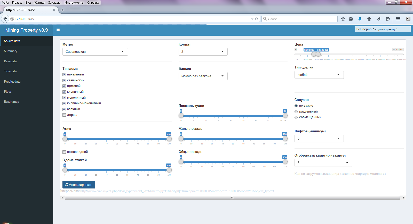
Fig. 1 Window of the selected menu Source data
In the remaining items of the side menu, the following is displayed:
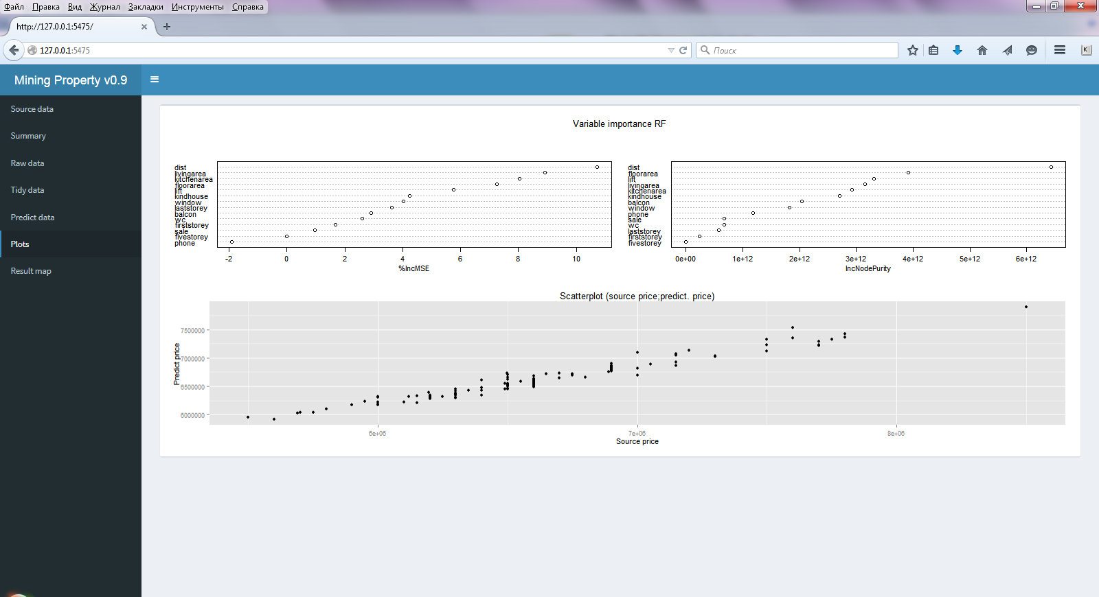
Fig.2 The window of the selected Plots menu
Well, in the last paragraph ( Result map ) (Fig. 3) you’ll see what it was all about, a map with the best results selected and a table with the calculated predicted price and the main characteristics of the apartments.
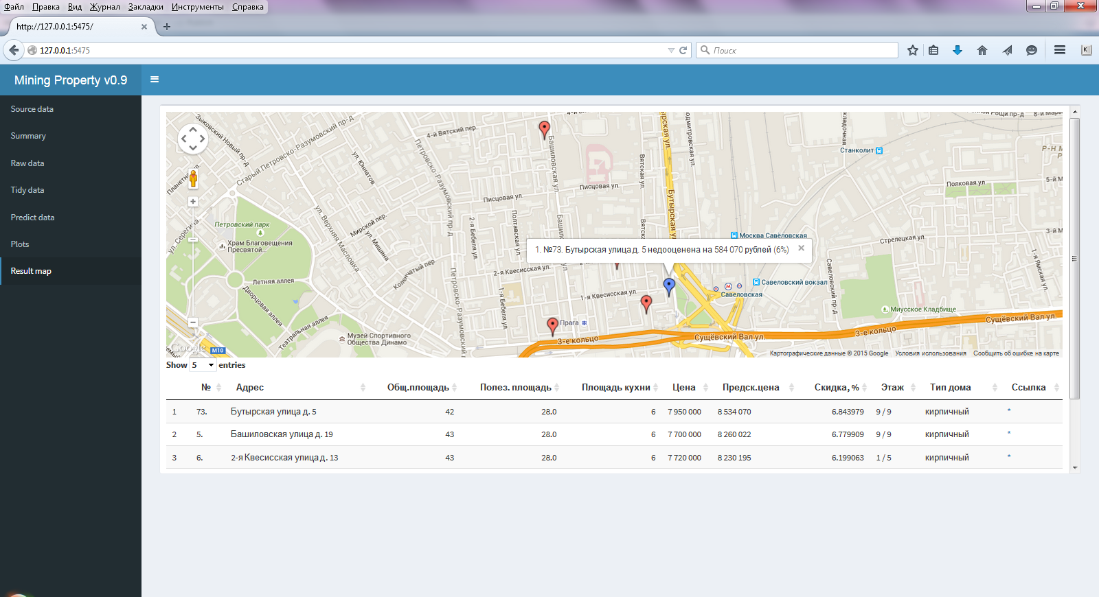
Fig. 3 Window of the selected Result map menu.
Also in this table there is immediately a link (*) to go to this announcement. This integration (inclusion of JS elements in the table) allows the DT package to be made .
Summarizing all of the above, how does it all work:
All the application’s work (from the beginning of the request to display on the map) is completed in less than a minute (most of the time is spent on geolocation, Google’s restriction for household use).
This publication wanted to show how, for simple household needs, within the framework of one application, it was possible to solve many small, but fundamentally different interesting subtasks:
In addition, all this is implemented in a convenient graphical application that can be either local or hosted on the network, and all this is done on one R (not counting import.io ), with a minimum of lines of code with a simple and elegant syntax. Of course, something is not taken into account, for example, the house near the highway or the condition of the apartment (since this is not in the ads), but the final, ranked list of options that are immediately displayed on the map and with a link to the original ad itself greatly simplifies the choice of apartments, Well, plus everything I learned a lot in R.
But this approach is time-consuming, inaccurate and will not allow to take into account all the variety of differences of apartments from each other. Therefore, I decided to automate the process of selecting real estate using data analysis by predicting a “fair” price. This publication describes the main stages of such an analysis, selects the best predictive model from eighteen tested models based on three quality criteria, as a result, the best (underestimated) apartments are immediately marked on the map, and all this using one web application created using R.Data collection
With the statement of the problem, it is clear, the question is where to get the data from, in Russia there are several main sites for finding real estate, and there is a WinNER database, which in a fairly convenient interface contains the maximum number of ads and allows uploading in csv format. But if earlier this base allowed time-based access (minutes, hours, days), now now the minimum is only 3 months of access, which is somewhat redundant for the average buyer or seller (although if you take it seriously, you can incur these costs). With this option, it would be quite simple, so let's go the other way, by parsing from some real estate site. From several options, I chose the most convenient notorious cian.ru. At that time, the data display was presented in a simple tabular form, but when I tried to parse all the data into R, then I failed. In some cells, the data could be incomplete, and with the standard means of the R functions I could not catch on anchor words or symbols, and I had to either use loops (which is incorrect for such a task in R) or use regular expressions that I am not familiar with at all , so I had to use an alternative. This alternative turned out to be a great service import.io , which allows you to retrieve information from pages (or sites), has its own REST API and returns a JSON result. And R can implement the request to the API and parse the JSON.
Having quickly mastered this service, I created an extractor on it, which extracts all the required information (all parameters of each apartment) from one page. And R already iterates over all pages, calling this API for each and gluing the received JSON data into a single table. Although import.io allows you to make a fully autonomous API that would go through all the pages, I decided that it’s logical that I can’t do it (parsing one page) correctly put on a third-party API, and continue to do the rest in R. So, the data source is selected, now about the limitations of the future model:
- Moscow city
- One type of apartment in the model (i.e. odnushki or dvushka or treshka)
- Within the same metro station (since geocoding is used, and the distance to the nearest metro)
- Resale (since new buildings are all fundamentally different, and are qualitatively different from each other, but this is either not said in the ads, or something is written in the comments, but neither one nor the other makes it possible to create an adequate model)
Data Overview
As often happens, the data may include emissions, gaps, and just a hoax when new buildings give out as a secondary, or even sell land.
Therefore, initially it is necessary to bring all the data to a "neat" look.
Cheat check
Here the main emphasis is on the description of the announcement, if there are words that are clearly not related to the sample I need, these observations are excluded, this is checked by the R grep function . And since the calculations are vector in R, this function immediately returns the vector of values of the correct observations, applying it, we filter the sample.
Check for missing values
Missed values are quite rare (and mainly in the “left” ads, with new buildings and land, which by this moment are already excluded), but with those that remain, something needs to be done. There are two options, in general, to exclude such observations or to replace these missing values. Since I didn’t want to sacrifice observations, but based on the assumption that the data is not filled on the basis of the principle “what to fill it in, and so it is clear that everything is like it”, I decided to replace qualitative variables with the mode of their values, and quantitative (footage) with median values. Of course, this is not entirely correct, and it would be completely correct to carry out a correlation relationship between the observations and fill in the gaps according to the results obtained, but for this task I considered this excessive, moreover, there are few such observations.
Emission check
Emissions are even less common, and can only be quantitative, namely in terms of price and footage. Here I proceeded from the assumption that the buyer (I) specifically knows at what price and approximately what footage his apartment should be, therefore, setting the initial values of the upper and lower prices, limiting the footage, we automatically get rid of emissions. But even if this is not so (do not make restrictions), then when you receive the result or by looking at the scattering diagram and seeing that there is an outlier, you can query with updated data, thereby removing these observations, which will improve the model.
Basic premises of the Gauss-Markov theorem
more details
So, we eliminated incorrect observations, then before conducting the analysis, we evaluate them on the main premises of the Gauss-Markov theorem.
Looking ahead, I’ll say that we don’t want the interpretation of the coefficients from the model, or the correct assessment of their confidence intervals, we need it to predict the “theoretical” price, so some of the premises are not critical for us.
The data are generally consistent with the assumptions, so you can build models.
Looking ahead, I’ll say that we don’t want the interpretation of the coefficients from the model, or the correct assessment of their confidence intervals, we need it to predict the “theoretical” price, so some of the premises are not critical for us.
- The data model is correctly specified. In general, yes, by eliminating outliers, incorrect announcements, replacing missing values, the model is quite adequate. Some non-strict multicollinearity may be present (for example, a five-story building and there is no elevator or area - common / residential), but as I wrote above, this is not critical for forecasting, moreover, it does not violate the basic premises. For the purpose of constructing test models, all values were correctly translated into dummy variables; strict multicollinearity was excluded.
- All regressors are deterministic and not equal. Yes, that’s also true.
- Errors are not systematic. It is true, since in the least-squares method a free term is used, which equalizes errors.
- The variance of errors is the same (homoskedasticity). Since restrictions on the size of the regressors and the dependent variable are used (the scale is comparable), heteroskedasticity is minimal, and again it is not critical for forecasting (standard errors are untenable, but they are not interesting to us)
- Errors are uncorrelated (endogenous). No, endogenousness, most likely, exists (for example, apartments are “neighbors” from one site or entrance), there is some external unaccounted factor, but again for forecasting, recording with endogenousity is not critical, moreover, we don’t know this unaccounted factor.
The data are generally consistent with the assumptions, so you can build models.
Regressors Set
In addition to the variables (obtained directly from the site), I decided to add additional regressors, namely a five-story house or not (since this is usually a very qualitative difference), and the distance to the nearest metro (similarly). To determine the distance, the Google geocoding service API is used (I chose it as the most accurate, loyal to restrictions, and there is a ready-made function in R), the addresses of apartments and the metro are geocoded first, using the geocode function from the ggmap package . And the distance is determined by the haversine formula, ready by the distHaversine function from the geosphere package .
The total number of regressors was 14 pieces:
- Distance to metro
- total area
- Living space
- Kitchen area
- House type
- Availability and types of elevators
- Availability and types of balconies
- Number and types of bathrooms
- Where do the windows go?
- Phone availability
- Type of sale
- Ground floor
- Top floor
- Five-story building
Tested Predictive Analysis Models
more details
In addition to practical personal value, it was also interesting to test different models, then I decided to select the best model to check various samples for all simple regression models that I know, namely, the following models were tested:
1. MNCs for all regressors
2. MNCs with logarithms (different options: by logarithm of the price and / or area and / or distance to the metro)
3. OLS with the inclusion and exclusion of regressors
a) sequential step-by-step exclusions of regressors
b) direct search algorithm
4. Models with fines (to reduce the influence of heteroskedasticity)
a) Lasso regression (with 2 methods for determining the fractionation parameter - minimizing the Cp criterion of Mallow and cross-checking)
b) Ridge regression (with 3 ways to find the penalty parameter - HKB, LW and cross-validation)
5. The main component method a
) with all regressors
b) with step-by-step exclusion of regressors
6. Quantile (median) regression (to reduce the effect of heteroskedasticity)
7. Random Forest Algorithm The
total number of tested models was 18.
In the process of preparing models, partially used materials:
Mastitsky S.E., Shitikov V.K. (2014) Statistical analysis and visualization of data using R.
- E-book, access address: r-analytics.blogspot.com
1. MNCs for all regressors
2. MNCs with logarithms (different options: by logarithm of the price and / or area and / or distance to the metro)
3. OLS with the inclusion and exclusion of regressors
a) sequential step-by-step exclusions of regressors
b) direct search algorithm
4. Models with fines (to reduce the influence of heteroskedasticity)
a) Lasso regression (with 2 methods for determining the fractionation parameter - minimizing the Cp criterion of Mallow and cross-checking)
b) Ridge regression (with 3 ways to find the penalty parameter - HKB, LW and cross-validation)
5. The main component method a
) with all regressors
b) with step-by-step exclusion of regressors
6. Quantile (median) regression (to reduce the effect of heteroskedasticity)
7. Random Forest Algorithm The
total number of tested models was 18.
In the process of preparing models, partially used materials:
Mastitsky S.E., Shitikov V.K. (2014) Statistical analysis and visualization of data using R.
- E-book, access address: r-analytics.blogspot.com
Model Performance Criteria
more details
All models are fundamentally different in nature, and for many of them there is no likelihood function, therefore, it is impossible to determine internal quality criteria, and it is not entirely correct to rely on them to select an effective model, since they primarily serve to assess the adequacy of the model. Therefore, we will focus on assessing the quality of models on the average difference between empirical and predicted values. And to make it more interesting, and to determine the benefit (cost-effectiveness), the root-mean-square error (as some observations may distort it) will not always be indicative, I used not only the usual RMSE - the standard error, but also MAE - the mean-square error, to evaluate the criteria and MPE, the average percentage error.
Model Test Results
more details
Since the models are evaluated by different functions and the syntax of the predicted values is also different, a simple indication that some regressors are factorial is not suitable for all models, so an additional data frame was created in which all qualitative variables were transformed into dummy variables and in this form models were built. This allows you to uniformly evaluate all models, predict new prices, and identify errors.
At various random test samples (different metro stations, different types of apartments, other parameters), all of the above models were evaluated by 3 performance criteria. And the almost absolute (92%) winner in all 3 criteria was the random forest algorithm. Also, on different samples, according to some criteria, median regression, OLS with a logarithm of prices, full OLS and sometimes Ridge with Lasso showed good results. The results are somewhat surprising, since I thought that models with penalties might turn out to be better than a full MNC, but this was not always the case. So a simple model (OLS) may be a better alternative than more complex ones. Due to the fact that in different samples, according to different criteria, the places starting from the second one were occupied by different models, and the winner was a random forest, I decided to use it for further work.
Since one model is already used, there is no need to explicitly specify dummy variables, so we return to the original frame, indicating that high-quality variables are factorial, this will simplify the subsequent interpretation on the diagram, and the algorithm will be easier (although it essentially doesn’t matter ) For test modeling, we used the randomForest function (from the package of the same name) with default values, trying to change the main complexity parameters of the nodesize , maxnodes , nPerm trees , determined that a slightly better minimization of forecast errors for different samples is achieved by changing the nodesize parameter (minimum number of nodes) in 1. So, the model is selected.
At various random test samples (different metro stations, different types of apartments, other parameters), all of the above models were evaluated by 3 performance criteria. And the almost absolute (92%) winner in all 3 criteria was the random forest algorithm. Also, on different samples, according to some criteria, median regression, OLS with a logarithm of prices, full OLS and sometimes Ridge with Lasso showed good results. The results are somewhat surprising, since I thought that models with penalties might turn out to be better than a full MNC, but this was not always the case. So a simple model (OLS) may be a better alternative than more complex ones. Due to the fact that in different samples, according to different criteria, the places starting from the second one were occupied by different models, and the winner was a random forest, I decided to use it for further work.
Since one model is already used, there is no need to explicitly specify dummy variables, so we return to the original frame, indicating that high-quality variables are factorial, this will simplify the subsequent interpretation on the diagram, and the algorithm will be easier (although it essentially doesn’t matter ) For test modeling, we used the randomForest function (from the package of the same name) with default values, trying to change the main complexity parameters of the nodesize , maxnodes , nPerm trees , determined that a slightly better minimization of forecast errors for different samples is achieved by changing the nodesize parameter (minimum number of nodes) in 1. So, the model is selected.
Map display
The winner is determined (random forest), this model predicts "theoretical" prices for all observations with minimal errors. Now you can calculate the absolute, relative underestimation and display the result in the form of a sorted table, but in addition to the tabular view, you want to immediately have information, so we’ll display some of the best results immediately on the map. And for this, R has a googleVis package designed for integration with the Google mapping system (however, there is a package for Leaflet as well). I continued to use Google as well, since the received coordinates from their geocoding are forbidden to be displayed on other maps. Display on the map is carried out by one function gvisMap from googleVis package .
map display code
output $ view <- renderGvis ({#view - output element htmlOutput
if ((err ()! = "")) return (NULL)
formap3 <-formap ()
formap3 $ desc <-paste0 (row.names (formap3),
". No.",
formap3 $ number,
"",
formap3 $ address,
"underestimated by",
format (-formap3 $ abs.discount, big.mark = ""),
"rubles (",
as.integer (formap3 $ otn .discount),
"%)")
gvisMap (formap3, "coord", "desc", options = list (
mapType = 'normal',
enableScrollWheel = TRUE,
showTip = TRUE))
})
if ((err ()! = "")) return (NULL)
formap3 <-formap ()
formap3 $ desc <-paste0 (row.names (formap3),
". No.",
formap3 $ number,
"",
formap3 $ address,
"underestimated by",
format (-formap3 $ abs.discount, big.mark = ""),
"rubles (",
as.integer (formap3 $ otn .discount),
"%)")
gvisMap (formap3, "coord", "desc", options = list (
mapType = 'normal',
enableScrollWheel = TRUE,
showTip = TRUE))
})
Web GUI
Passing all the required parameters through the console is slow and inconvenient, so I wanted to do everything automatically. And traditionally, for this you can again use R with the shiny and shinydashboard frameworks , which have sufficient I / O controls.
full code of the client part of the interface
dashboardPage (
dashboardHeader (title = "Mining Property v0.9"),
dashboardSidebar (
sidebarMenu (
menuItem ("Source data", tabName = "Source"),
menuItem ("Summary", tabName = "Summary"),
menuItem ("Raw data ", tabName =" Raw "),
menuItem (" Tidy data ", tabName =" Tidy "),
menuItem (" Predict data ", tabName =" Predict "),
menuItem (" Plots ", tabName =" Plots ") ,
menuItem (“Result map”, tabName = “Map”)
)
),
dashboardBody (
tags $ head (tags $ style (HTML ('. box {overflow: auto;}'))),
tabItems (
tabItem ("Source" ,
box (width = 12,
fluidRow (
column (width = 4,
selectInput ("Metro", "Metro", "", width = '60% '),
# br (),
hr (),
#checkboxInput ("Kind.home0", "all", TRUE),
checkboxGroupInput ("Kind .home ”,“ House type ”, c (
“ panel ”= 1,
“ Stalin ”= 7,
“ panel ”= 8,
“ brick ”= 2,
“ monolithic ”= 3,
“ brick-monolithic ”= 4,
“ block "= 5,
" tree "= 6), selected = c (1,2,3,4,5,6,7,8)),
hr (),
sliderInput (" Etag "," Floor ", min = 0, max = 100, value = c (0, 100), step = 1),
checkboxInput (“EtagP”, “not the last”),
sliderInput (“Etagn”, “In the house of floors”, min = 0, max = 100, value = c (0, 100), step = 1)
,
submitButton (“Analyze”, icon (“refresh”))
),
column (width = 4,
selectInput ("Rooms", "Rooms", c
("",
"1" = "& room1 = 1",
"2" = "& room2 = 1",
"3" = "& room3 = 1" ), width = '45% '),
# br (),
hr (),
# br (),
selectInput ("Balcon", "Balcony",
c ("can be without a balcony" = "0",
"only with a balcony "=" & Minbalkon = 1 ",
" only without a balcony "=" & minbalkon = -1 "),
width = '45% '),
br (),
hr (),
br (),
#br (),
sliderInput (" KitchenM ”,“ Kitchen Area ”, min = 0, max = 25, value = c (0, 25), step = 1),
sliderInput (“ GilM ”,“ Living Area ”, min = 0, max = 100, value = c (0, 100), step = 1),
sliderInput (“TotalM”, “Totalarea ”, min = 0, max = 150, value = c (0, 150), step = 1)
),
column (width = 4,
sliderInput ("Price", "Price", min = 0, max = 50000000, value = c (0, 50000000), step = 100000, sep = ""),
# hr (),
selectInput ("Deal", "Transaction Type",
c ("any" = "0",
"free" = "& sost_type = 1",
"alternative" = "& sost_type = 2"),
width = '45% ') ,
br (),
hr (),
#br (),
# br (),
# br (),
radioButtons ("wc", "Bathroom",
c ("not important" = "",
"separate" = "& minsu_r = 1 ",
" combined "=" & minsu_s = 1 ")),
hr (),
selectInput (" Lift "," Lifts (minimum) ",
c (" 0 "= 0,
" 1 "=" & minlift = 1 " ,
"2" = "& minlift = 2",
"3" = "& minlift = 3",
“4” = “& minlift = 4”
),
width = '45% '),
hr (),
selectInput (“obs”, “Display apartments on the map:”, c (1:10), selected = 5, width = 250),
textOutput ("flat")
)
),
fluidRow (htmlOutput ("hyperf1")),
fluidRow (textOutput ("testOutput"))
)
),
tabItem ("Raw", box (dataTableOutput ("Raw"), width = 12, height = 600)),
tabItem ("Summary", box (verbatimTextOutput ("Summary"), width = 12, height = 600)),
tabItem ("Tidy", box (dataTableOutput ("Tidy"), width = 12, height = 600)),
tabItem ("Predict", box (dataTableOutput ("Predict"), width = 12, height = 600)),
tabItem ("Plots", box (width = 12, plotOutput ("RFplot ", Height = 275), plotOutput (" r2 ", height = 275))),
tabItem ("Map", box (width = 12, htmlOutput ("view"), DT :: dataTableOutput ("formap2"), height = 600))
)
)
)
dashboardHeader (title = "Mining Property v0.9"),
dashboardSidebar (
sidebarMenu (
menuItem ("Source data", tabName = "Source"),
menuItem ("Summary", tabName = "Summary"),
menuItem ("Raw data ", tabName =" Raw "),
menuItem (" Tidy data ", tabName =" Tidy "),
menuItem (" Predict data ", tabName =" Predict "),
menuItem (" Plots ", tabName =" Plots ") ,
menuItem (“Result map”, tabName = “Map”)
)
),
dashboardBody (
tags $ head (tags $ style (HTML ('. box {overflow: auto;}'))),
tabItems (
tabItem ("Source" ,
box (width = 12,
fluidRow (
column (width = 4,
selectInput ("Metro", "Metro", "", width = '60% '),
# br (),
hr (),
#checkboxInput ("Kind.home0", "all", TRUE),
checkboxGroupInput ("Kind .home ”,“ House type ”, c (
“ panel ”= 1,
“ Stalin ”= 7,
“ panel ”= 8,
“ brick ”= 2,
“ monolithic ”= 3,
“ brick-monolithic ”= 4,
“ block "= 5,
" tree "= 6), selected = c (1,2,3,4,5,6,7,8)),
hr (),
sliderInput (" Etag "," Floor ", min = 0, max = 100, value = c (0, 100), step = 1),
checkboxInput (“EtagP”, “not the last”),
sliderInput (“Etagn”, “In the house of floors”, min = 0, max = 100, value = c (0, 100), step = 1)
,
submitButton (“Analyze”, icon (“refresh”))
),
column (width = 4,
selectInput ("Rooms", "Rooms", c
("",
"1" = "& room1 = 1",
"2" = "& room2 = 1",
"3" = "& room3 = 1" ), width = '45% '),
# br (),
hr (),
# br (),
selectInput ("Balcon", "Balcony",
c ("can be without a balcony" = "0",
"only with a balcony "=" & Minbalkon = 1 ",
" only without a balcony "=" & minbalkon = -1 "),
width = '45% '),
br (),
hr (),
br (),
#br (),
sliderInput (" KitchenM ”,“ Kitchen Area ”, min = 0, max = 25, value = c (0, 25), step = 1),
sliderInput (“ GilM ”,“ Living Area ”, min = 0, max = 100, value = c (0, 100), step = 1),
sliderInput (“TotalM”, “Totalarea ”, min = 0, max = 150, value = c (0, 150), step = 1)
),
column (width = 4,
sliderInput ("Price", "Price", min = 0, max = 50000000, value = c (0, 50000000), step = 100000, sep = ""),
# hr (),
selectInput ("Deal", "Transaction Type",
c ("any" = "0",
"free" = "& sost_type = 1",
"alternative" = "& sost_type = 2"),
width = '45% ') ,
br (),
hr (),
#br (),
# br (),
# br (),
radioButtons ("wc", "Bathroom",
c ("not important" = "",
"separate" = "& minsu_r = 1 ",
" combined "=" & minsu_s = 1 ")),
hr (),
selectInput (" Lift "," Lifts (minimum) ",
c (" 0 "= 0,
" 1 "=" & minlift = 1 " ,
"2" = "& minlift = 2",
"3" = "& minlift = 3",
“4” = “& minlift = 4”
),
width = '45% '),
hr (),
selectInput (“obs”, “Display apartments on the map:”, c (1:10), selected = 5, width = 250),
textOutput ("flat")
)
),
fluidRow (htmlOutput ("hyperf1")),
fluidRow (textOutput ("testOutput"))
)
),
tabItem ("Raw", box (dataTableOutput ("Raw"), width = 12, height = 600)),
tabItem ("Summary", box (verbatimTextOutput ("Summary"), width = 12, height = 600)),
tabItem ("Tidy", box (dataTableOutput ("Tidy"), width = 12, height = 600)),
tabItem ("Predict", box (dataTableOutput ("Predict"), width = 12, height = 600)),
tabItem ("Plots", box (width = 12, plotOutput ("RFplot ", Height = 275), plotOutput (" r2 ", height = 275))),
tabItem ("Map", box (width = 12, htmlOutput ("view"), DT :: dataTableOutput ("formap2"), height = 600))
)
)
)
The result of all this is a convenient application with a graphical interface, with actually two (other items for control) main points of the side menu - the first and the last. In the first ( Source data ) item of the side menu (Fig. 1), all the required parameters (similar to cian) for searching and evaluating apartments are set.
Fig. 1 Window of the selected menu Source data
In the remaining items of the side menu, the following is displayed:
- Synthesis Report ( Summary A ) of regressors
- data tables ( Raw (raw data ) - initial after parsing, neat ( Tidy data ) - after bringing the parameters into a neat appearance and adjusting the parameters and adding geolocation, and the final ( Predict data ) table with the predicted price values)
- three Plots diagrams ( Fig. 2) - the accuracy of the model and the importance of the regressors in the random forest algorithm (almost always all regressors are important) and the dispersion diagram of the initial and predicted prices.
Fig.2 The window of the selected Plots menu
Well, in the last paragraph ( Result map ) (Fig. 3) you’ll see what it was all about, a map with the best results selected and a table with the calculated predicted price and the main characteristics of the apartments.
Fig. 3 Window of the selected Result map menu.
Also in this table there is immediately a link (*) to go to this announcement. This integration (inclusion of JS elements in the table) allows the DT package to be made .
Conclusion
Summarizing all of the above, how does it all work:
- On the first page, the initial request is set using controls
- Based on the selection of these input elements, a query string is generated (it is also indicated as a hyperlink for verification)
- This line indicating the page is passed to the import.io API (in the process of creating all this, cian started changing the output interface, thanks to import.io I retrained the extractor in literally 5 minutes)
- Received JSON from API is processed
- All pages are scanned (in the process, a status bar is displayed for the processes)
- Tables are glued together, checked (incorrect values are excluded, missing values are replaced), brought into a uniform form suitable for analysis
- Geocoding addresses and determining distance
- The model is constructed according to the random forest algorithm
- The predicted prices, absolute, relative deviations are determined
- The best results are displayed on the map and in the table below it (the number of displayed apartments is indicated on the first page)
All the application’s work (from the beginning of the request to display on the map) is completed in less than a minute (most of the time is spent on geolocation, Google’s restriction for household use).
This publication wanted to show how, for simple household needs, within the framework of one application, it was possible to solve many small, but fundamentally different interesting subtasks:
- crowing
- parsing
- 3rd party API integration
- JSON processing
- geocoding
- work with various regression models
- assessment of their effectiveness in different ways
- geolocation
- map display
In addition, all this is implemented in a convenient graphical application that can be either local or hosted on the network, and all this is done on one R (not counting import.io ), with a minimum of lines of code with a simple and elegant syntax. Of course, something is not taken into account, for example, the house near the highway or the condition of the apartment (since this is not in the ads), but the final, ranked list of options that are immediately displayed on the map and with a link to the original ad itself greatly simplifies the choice of apartments, Well, plus everything I learned a lot in R.