Conjugation tables and factorization of non-negative matrices
The non-negative matrix factorization (NMF) is a representation of the matrix V as a product of the matrices W and H , in which all elements of the three matrices are non-negative. This decomposition is used in various fields of knowledge, for example, in biology, computer vision, recommendation systems. This publication will discuss the contingency tables of sociological and marketing data, the factorization of which helps to understand the data structure of these tables.

Surprisingly, apparently, they did not write about NMF on Habré yet. The history of this method and general information are available on Wikipedia . But first, we will answer the question why do we need to convert contingency tables in any way.
If the number of rows and columns in the table is small, then a simple chart with columns or a stacked bar chart is enough to have an idea of the data in the table. For example, a table obtained by the intersection of the variables “gender” and “frequency of visits to sports or fitness clubs over the past month (4 categories)” of size 2x4 can be easily analyzed. Another thing is if the size of the table grows, say up to 20x30 or more. In the jungle of the numbers in the table and in the forest of columns of the graph, it will be impossible or extremely difficult to detect patterns. In this case, the alternative is NMF, which lowers the dimension of the contingency table and displays the result in the form of heat maps. This gives an extremely visual and easily interpreted view of the table.
Historically, one of the first methods for graphically representing the structure of a transformed table is correspondence analysis (CA). It goes back to the principal component method, and is based on singular matrix decomposition (SVD). You can read about SVD in this article on Habré. It also mentions an excellent video with SVD definition and an example of building correspondence analysis. Correspondence analysis is a popular method, but factorization of non-negative matrices, in my opinion, has several advantages. Considerations for this will be presented at the end of this article.
The following are only those definitions of factorization that are necessary for the analysis of contingency tables. Let table V have size mxn . Denote by rthe rank of the matrices W and H , as a rule, r << min (n, m) . Unlike the exact representation of the matrix in SVD, in NMF we have only approximate equality

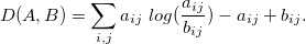
The matrices W and H are chosen in such a way as to minimize the loss function: D (V, WH) -> min. In our case, D is set based on the Kullback-Leibler divergence
The question remains with the choice of rank r. There are several methods for estimating r (as, for example, in the case of the parameter k in the k- averages method ). But it is better to leave the choice of r to the discretion of the researcher / user, the rank at which the structure of the tables is most understandable, simple, appropriate, and optimal.
In the R environment, there is a package nmf [1], which implements several algorithms for factorization of non-negative matrices, visualization of decomposition, and its diagnostics. The capabilities of NMF will be demonstrated on data from Round 6 of the European Social Research (ESS) . A previous publication showed how you can load this data into R.
The 2012 ESS project was attended by 29 countries. The questionnaire, in particular, included 21 questions about the degree of importance of human values with a scale of six values: from “Very much like me” to “Not like me at all”. We transform each of these 21 single response variables into a logical variable. This variable accepts True for those respondents for whom this value is important - “Very much like me” and “Like me”; for all other respondents - doubters, for those who do not share this value or who do not answer, the variable takes the value False.
Define the general population as “Men aged 20-45 years.” We construct a table of intersections of these logical variables with each of the 29 countries of the study, taking into account the weights of the respondents. We get a table of size 29x21.
Please note that the contingency table is perceived in an expanded sense, it contains a multiple response variable about human values. In addition, the size of the gene. the populations in each country are different. Due to these two features of the table, it is important to normalize its rows to the size of the gene. populations of countries. That is, the table consists of weighted average values of support values in each country of the ESS study. This is her fragment

Now construct the heat! Matrices W and H . They determine the decomposition of the studied characteristics in the space of 5 latent variables. The darker the cell, the more pronounced is the correspondence between the latent variable and the value or country. I omit the mathematical details of an exact definition; details can be found in [1].
Next, we select only those human.values variables that are expressed only along one of the axes in this space. The names of the axes are given by me independently.

The final result is shown below, representing all 29 countries. The degree of correspondence of variables is expressed in color. In addition, countries are grouped according to hierarchical clustering with the Euclidean metric in the 5-dimensional space of latent variables.
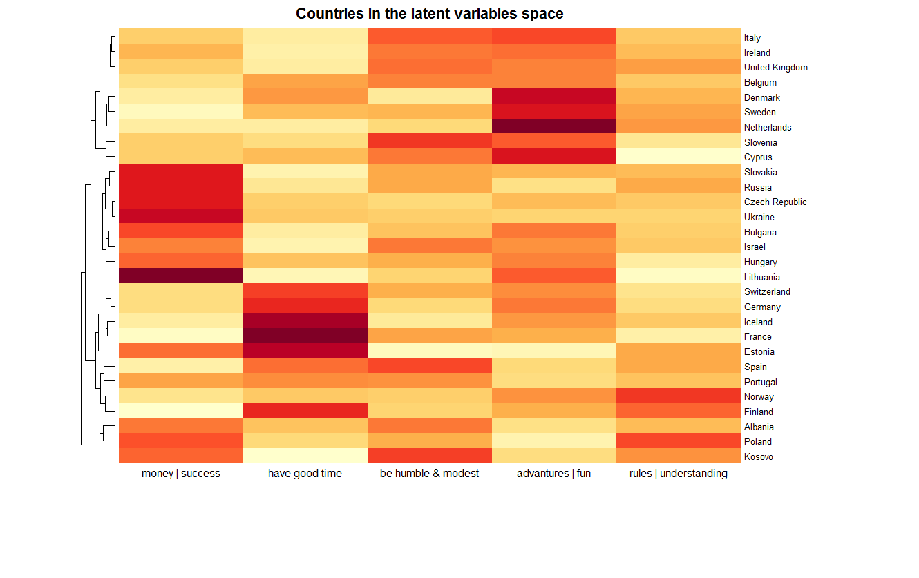
We see that in this space the closest country to Russia is Slovakia. These countries, in particular, are distinguished by their severity along the first axis, which cannot be said, for example, about France. This point will be considered in more detail in the next part of the article. The chart also shows which countries make up the clusters, depending on the details required. For example, a cluster from Eastern Europe (Slovakia, Russia, Czech Republic, Ukraine, Bulgaria, Hungary, Lithuania) and Israel. A curious cluster from Albania, Kosovo and ... Poland. And Norway and Finland are quite far located from Denmark with Sweden.
The use of NMF for marketing contingency tables can be found in this publication . It considers an example of analysis of the perception of 14 automobile brands.
NMF diagrams, no matter how good they are, in general, do not give reason to draw conclusive conclusions about the similarities and differences of different countries regarding ideas about values. This problem will be considered in the next part of the article.
References:
[1] Renaud Gaujoux et al. A flexible R package for nonnegative matrix factorization. In: BMC Bioinformatics 11.1 (2010), p. 367.
Surprisingly, apparently, they did not write about NMF on Habré yet. The history of this method and general information are available on Wikipedia . But first, we will answer the question why do we need to convert contingency tables in any way.
If the number of rows and columns in the table is small, then a simple chart with columns or a stacked bar chart is enough to have an idea of the data in the table. For example, a table obtained by the intersection of the variables “gender” and “frequency of visits to sports or fitness clubs over the past month (4 categories)” of size 2x4 can be easily analyzed. Another thing is if the size of the table grows, say up to 20x30 or more. In the jungle of the numbers in the table and in the forest of columns of the graph, it will be impossible or extremely difficult to detect patterns. In this case, the alternative is NMF, which lowers the dimension of the contingency table and displays the result in the form of heat maps. This gives an extremely visual and easily interpreted view of the table.
Historically, one of the first methods for graphically representing the structure of a transformed table is correspondence analysis (CA). It goes back to the principal component method, and is based on singular matrix decomposition (SVD). You can read about SVD in this article on Habré. It also mentions an excellent video with SVD definition and an example of building correspondence analysis. Correspondence analysis is a popular method, but factorization of non-negative matrices, in my opinion, has several advantages. Considerations for this will be presented at the end of this article.
The following are only those definitions of factorization that are necessary for the analysis of contingency tables. Let table V have size mxn . Denote by rthe rank of the matrices W and H , as a rule, r << min (n, m) . Unlike the exact representation of the matrix in SVD, in NMF we have only approximate equality
The matrices W and H are chosen in such a way as to minimize the loss function: D (V, WH) -> min. In our case, D is set based on the Kullback-Leibler divergence
The question remains with the choice of rank r. There are several methods for estimating r (as, for example, in the case of the parameter k in the k- averages method ). But it is better to leave the choice of r to the discretion of the researcher / user, the rank at which the structure of the tables is most understandable, simple, appropriate, and optimal.
In the R environment, there is a package nmf [1], which implements several algorithms for factorization of non-negative matrices, visualization of decomposition, and its diagnostics. The capabilities of NMF will be demonstrated on data from Round 6 of the European Social Research (ESS) . A previous publication showed how you can load this data into R.
The 2012 ESS project was attended by 29 countries. The questionnaire, in particular, included 21 questions about the degree of importance of human values with a scale of six values: from “Very much like me” to “Not like me at all”. We transform each of these 21 single response variables into a logical variable. This variable accepts True for those respondents for whom this value is important - “Very much like me” and “Like me”; for all other respondents - doubters, for those who do not share this value or who do not answer, the variable takes the value False.
Define the general population as “Men aged 20-45 years.” We construct a table of intersections of these logical variables with each of the 29 countries of the study, taking into account the weights of the respondents. We get a table of size 29x21.
Please note that the contingency table is perceived in an expanded sense, it contains a multiple response variable about human values. In addition, the size of the gene. the populations in each country are different. Due to these two features of the table, it is important to normalize its rows to the size of the gene. populations of countries. That is, the table consists of weighted average values of support values in each country of the ESS study. This is her fragment
Code for constructing a table and finding its factorization of rank 5.
The research data has already been downloaded, the names of the objects have remained unchanged.
We list the names of the variables in the study base corresponding to questions about human values
We add to the database logical variables converted to a numeric type and multiplied by the respondents' weights
Build the required table (denoted by cntry.human.values)
And we factorize non-negative rank 5 matrices
We list the names of the variables in the study base corresponding to questions about human values
human.values <- c("ipcrtiv", "imprich", "ipeqopt", "ipshabt", "impsafe", "impdiff", "ipfrule",
                              "ipudrst", "ipmodst", "ipgdtim", "impfree", "iphlppl", "ipsuces", "ipstrgv",
                              "ipadvnt", "ipbhprp", "iprspot", "iplylfr", "impenv", "imptrad", "impfun")
We add to the database logical variables converted to a numeric type and multiplied by the respondents' weights
weighted.human.values<-paste(human.values,"w",sep="_")
add.binary.human.values<-function(){
  adding.variables<-paste("srv.data[,c('", paste(weighted.human.values, collapse = "','"), "'):=list(",
                               paste("as.numeric(",human.values, " %in% c( 'Very much like me', 'Like me' ))
                               *dweight", collapse = ", " ), ")]", sep="")
  eval(parse(text=adding.variables))
return(T)
}
add.binary.human.values()
Build the required table (denoted by cntry.human.values)
target.audience.data <- srv.data[gndr == 'Male' & agea >= 25 & agea<=40,
                                                    c(weighted.human.values,'dweight', 'cntry'), with=FALSE]
cntry.human.values <- t(sapply(unique(target.audience.data[,cntry]), function(x)
                                    colSums(target.audience.data[J(x)][,weighted.human.values,with=FALSE])))
cntry.pop.sizes <- target.audience.data[,list(W.Total=sum(dweight)),by=cntry]
cntry.human.values <- cntry.human.values/cntry.pop.sizes[,W.Total]*100
rownames(cntry.human.values) <- c("Albania", "Belgium", "Bulgaria", "Switzerland", "Cyprus",
                                               "Czech Republic", "Germany", "Denmark", "Estonia", "Spain",
                                               "Finland", "France", "United Kingdom", "Hungary", "Ireland",
                                               "Israel", "Iceland", "Italy", "Lithuania", "Netherlands", "Norway",
                                               "Poland", "Portugal", "Russia", "Sweden", "Slovenia", "Slovakia",
                                               "Ukraine", "Kosovo")
colnames(cntry.human.values) <- sub(srv.variables[J(human.values)][,title],
                                                      pattern = "Important to |Important that ", replacement = "")
And we factorize non-negative rank 5 matrices
nmf.fit <- nmf(cntry.human.values, 5, method = "brunet", seed=123456, nrun=100)
Now construct the heat! Matrices W and H . They determine the decomposition of the studied characteristics in the space of 5 latent variables. The darker the cell, the more pronounced is the correspondence between the latent variable and the value or country. I omit the mathematical details of an exact definition; details can be found in [1].
Next, we select only those human.values variables that are expressed only along one of the axes in this space. The names of the axes are given by me independently.
Building a profile map
nmf.selected <- nmf.fit[, c(2, 7:10, 13, 15, 21)]
basismap(t(nmf.selected), tracks=NA, main="Latent variables: Profiles explanation",
         scale = "r1", legend = NA,  Rowv=TRUE,  labCol = c("money | success",
        "have good time", "be humble & modest", "advantures | fun", "rules | understanding"))
The final result is shown below, representing all 29 countries. The degree of correspondence of variables is expressed in color. In addition, countries are grouped according to hierarchical clustering with the Euclidean metric in the 5-dimensional space of latent variables.
Hidden text
basismap (nmf.selected, tracks = NA, main = "Countries in the latent variables space",
legend = NA, labCol = c ("money | success", "have good time", "be humble & modest",
"advantures | fun "," rules | understanding "))
legend = NA, labCol = c ("money | success", "have good time", "be humble & modest",
"advantures | fun "," rules | understanding "))
We see that in this space the closest country to Russia is Slovakia. These countries, in particular, are distinguished by their severity along the first axis, which cannot be said, for example, about France. This point will be considered in more detail in the next part of the article. The chart also shows which countries make up the clusters, depending on the details required. For example, a cluster from Eastern Europe (Slovakia, Russia, Czech Republic, Ukraine, Bulgaria, Hungary, Lithuania) and Israel. A curious cluster from Albania, Kosovo and ... Poland. And Norway and Finland are quite far located from Denmark with Sweden.
Comparison with match analysis results
What are the benefits of NMF?
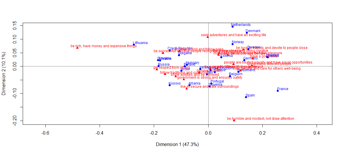
- Unlike NMF, in the graphical representation of the classical analysis of correspondence only two eigenvalues are used (in the graph above, the cumulative inertia of the CA axes is 57.4%). In NMF, visualization is also visible for a rank greater than two.
- Secondly, heatmaps present information in a more structured and visual way than the CA plane.
library(ca)
plot(ca(cntry.human.values), what=c("all", "active"))
What are the benefits of NMF?
- Unlike NMF, in the graphical representation of the classical analysis of correspondence only two eigenvalues are used (in the graph above, the cumulative inertia of the CA axes is 57.4%). In NMF, visualization is also visible for a rank greater than two.
- Secondly, heatmaps present information in a more structured and visual way than the CA plane.
The use of NMF for marketing contingency tables can be found in this publication . It considers an example of analysis of the perception of 14 automobile brands.
NMF diagrams, no matter how good they are, in general, do not give reason to draw conclusive conclusions about the similarities and differences of different countries regarding ideas about values. This problem will be considered in the next part of the article.
References:
[1] Renaud Gaujoux et al. A flexible R package for nonnegative matrix factorization. In: BMC Bioinformatics 11.1 (2010), p. 367.