Creating the Droste effect in Wolfram Language (Mathematica) / Wolfram Research Blog

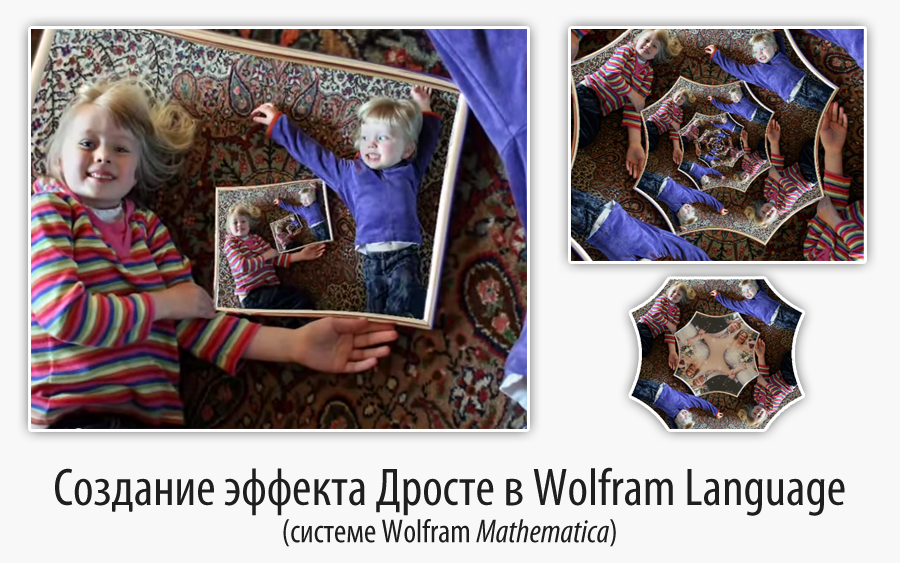
A translation of John MacLoon's post " Droste Effect with Mathematica ". The code in the article can be downloaded at the end of the post.
I express my deep gratitude to Kirill Guzenko for help with the translation.

---

The Droste effect ( wiki ) is a recursive inclusion of an image into itself. The name comes from the Droste cocoa powder, which was sold in 1904 in a package that depicted a nurse holding a box with a nurse on it, and so on. The simplest implementation is to scale and transform the image, and then place it on your unmodified exact copy, then start the process again. Take a look at a demo that uses original Droste packaging illustrations. However, much more interesting results can be achieved by using the theory of functions of a complex variable (TFKP). Escher M.K. was the first to popularize the idea of conformal mappingsin relation to images, however, with the help of computers, we can easily realize this idea in photographs to get something like this:



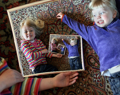
Yes, the idea is not new. However, when I decided to implement a similar effect, the methods that I found on the network seemed unsatisfactory to me. Some suggested a lot of copy-paste type of work on the images, while others had problems with the resolution mismatch at the joints of the parts of the images. And, as usual, I came to the conclusion that we need to use Mathematica , or in this case grid Mathematica .

In essence, the idea is simple. We create an image where the pixel at position { x, y } of the resulting image is obtained from the pixel at position f [{ x, y}] of our original image. The magic is to choose the function f itself . But before we get to this, we need to prepare something.

Currently, Mathematica does not contain operations for arbitrary transformation of images, so for starters I have to implement them ( Post written by John in the 7th version of Wolfram Mathematica, in the 8th version a special function ImageTransformation appeared for these purposes , which significantly reduces the amount of code in an article by John - approx.) The important point is to constantly calculate the color between the pixels to prevent resolution matching problems and unnecessary pixelation in enlarged areas of the image. My method is to linearly interpolate all the colors of the pixels in each RGB channel for the image. This is the most computationally complex approach, especially with the original images of 10 megapixels, but it gives me the quality I need.



To compensate for this approach, I set everything up for parallel computing. To get started, I used the parallelization tools built into Mathematica . Thus, instead of just using Table to generate a grid of pixels, I created a function that calls Tableto generate a layer of the final image, which is called in parallel by ParallelTable to redistribute the work between several processor cores. So 3-4 lines more, but this is only half the work of parallelization.





Then, I pass the original image to each processor and set the interpolation function. This part is very demanding on calculations, so I want to do this only once and after that be able to make any kind of image from the source without having to do this job again. Parallelization is quite simple here: the available kernels are launched, the program definition is distributed to all the kernels, and then the ParallelEvaluate function is usedto send an image via a link with a request to create an interpolation function.



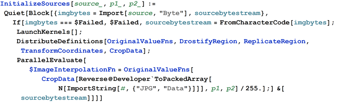
There is a graceful technique in transmitting an image as a string with the contents of a JPG file instead of transmitting real uncompressed data. It turns out a much smaller object, which, accordingly, is transmitted faster.

With this setup, I can easily attract additional computer cores from my office to speed up the calculations using grid Mathematica .

There’s something else to add to the code. So I get rid of the need for the original image to be cropped in the correct ratio and with the correct centering.



Here's what my original image looks like after cropping:



Well, everything is boring behind, now it's time to have fun.

The twisting that I use is based on the specific properties of the Power function on the complex plane. We can represent our coordinate pairs { x, y } as parts of a complex number p = x + I y , use the map f [ p ]: = p ^c, and return back to the Cartesian coordinates. It’s quite difficult to figure out how to take the value of c , especially if you use the more general model a + ( b + c p ) ^d , where { a, b, c, d} are complex numbers. So I decided to turn to the Wolfram Demonstrations Project, found a demonstration with conformal mappings there and changed the code a bit to get the mapping that interests me.

Having experimented, I found out the influence of the parameters, set up the calibration, got good initial values ​​and set the named options in the necessary places of the same magic formula. In the end, I got such a design for twisting.



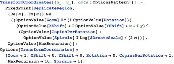
I provide this kind of self-reproduction by jumping inward when trying to access a pixel outside the image, and then outward while gaining access to a pixel inside a certain area.

For reasons of aesthetics, I would like to close the connections between the images to make them more natural. In my example, I used a picture frame, but I met examples where doorways, windows, computer monitors, and the like were used.

Automation of this process avoids manual copying and subsequent paste, and also avoids problems with the mismatch of the resolutions of various parts of the image.



Everything, all the laborious work is already behind, now is the time to indulge. Initialize the kernels with the original image by setting the coordinates of the inner area (you can easily get them using the coordinate picker in the 2D Drawing palette ):



Now we generate an image 400 pixels high:



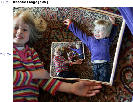
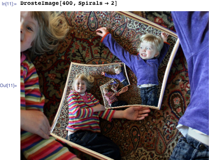
There are many combinations of parameters, for example, this one with a double spiral:



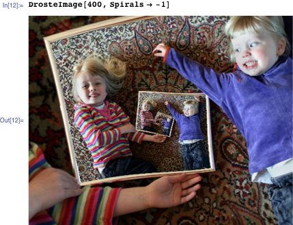
One spiral in the opposite direction:



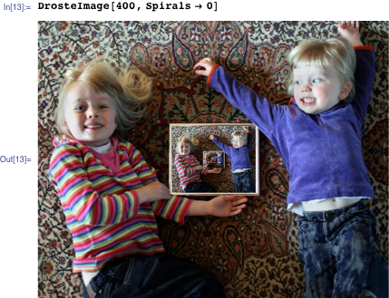
No spirals, only replication:



This code creates octagons by creating two copies per spiral:



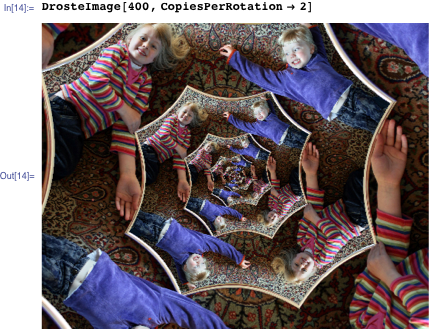
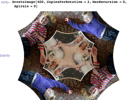
And this one without recursion and spirals - just two copies rolled up together:



And here, the climax is a whole film in DVD quality, showing the Droste effect of twisting the image into a recursive spiral.



Creating such a video requires a lot of calculations - calling three interpolation functions for each of 10 million pixels about 400 thousand times for each of 60 frames. This is the moment when my parallelization efforts really pay off. Of course, while at Wolfram Research, I have several grid Mathematica licenses at hand , communicating through the Wolfram Lightweight Grid Manager ( Starting with version 7 of Wolfram Mathematica, parallelization functionality is included in the Wolfram Language core and does not require additional programs when working, it is able to use all the kernels available on your computer, however, if you need to connect to the cluster, gridMathematica is required for this - approx.) I open Parallel Configuration preferences and they all magically appear. A few clicks, and now I have 16 more cores, in addition to two on my small laptop, and without any changes in the code, the movie is generated 8 times faster (and 16 times faster than without parallelization). I don’t know exactly where this code works, but since the program and source images are transferred automatically, it’s not very interesting for me. You can watch a screen demonstration of how this is all set up .



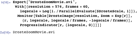
This code can be modified in different ways; e.g. change ReplicateRegionallows you to use non-rectangular frames, in the form of circles, for example, or you can even change the colors and transparency of replications. Try experimenting yourself and see what can come of it.