Software renderer - 2: attribute rasterization and interpolation
Hey. In a previous article, I described the mathematics that are needed to display a three-dimensional scene on the screen in the form of a grid - i.e. we stopped at the moment of obtaining the coordinates of the vertices in the screen space. The next step is to "fill" the polygons that make up the object, i.e. search for pixels that enter the image of the object on the screen. The process of finding these points is called rasterization. We also want to be able to texture and illuminate objects - for this it is necessary to be able to interpolate the attributes specified at the vertices (for example, texture coordinates, normals, color, and others).
Our input is a set of polygons (we will only consider triangles): the coordinates of their vertices (the coordinate system depends on the algorithm) and the attribute values at each of these vertices, which will be further interpolated along the surface of the triangle. There are several pitfalls that I will cover in this article:
I will consider three approaches to rasterization:
Also at the end there will be a link to the project, which is an example of implementation, from there will also be code examples.
So, rasterization is the process of finding pixels that are “included” in a given polygon. To begin with, we will assume that it is enough for us to fill the polygon with a solid color - nothing more.
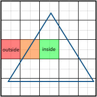
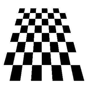
Imagine that we have the following triangle for displaying on the screen (all coordinates are already presented in the screen space):

What pixels need to be painted over? A pixel can be entirely outside the polygon, partially in the polygon and entirely in the polygon:
Everything is simple for two cases:
The third case (the pixel is partially inside the polygon) is more complicated. The first decision that comes to mind is to assume that all such pixels are either included in the polygon or not. But it leads to the wrong result. The three-dimensional models that we are going to draw consist of many triangles, which, in general, should not overlap each other. Triangles overlapping each other do not make sense, since they only duplicate existing information. Thus, many polygons have common faces. The simplest example is a rectangle:
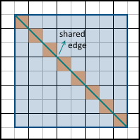
Pixels that partially fit into both polygons are marked in orange. Now imagine that we will rasterize both of these polygons. If we decide that all the pixels partially included in the polygon should be filled, we will get the same pixels twice (or more if there is a common vertex for more than two polygons). This may not seem like a problem at first glance, but in fact, it will lead to various artifacts when using some techniques, such as alpha blending (rendering using the alpha channel to simulate transparency). This also leads to a decrease in productivity, because the number of pixels for which we need to calculate attribute values is increasing. If, on the contrary, we decide that such pixels are not included in the final image and should not be filled,
Thus, we came to the understanding that each pixel when filling adjacent polygons must be filled exactly once. This is a requirement that both Direct3D and OpenGL comply with.
The problem arises from the need to display from continuous (screen coordinate system) to discrete (pixels on the monitor). The traditional rasterization algorithm (when rendering without smoothing) solves this as follows: each pixel is associated with a certain point (sample point), which is responsible for the pixel entering the polygon. Also, it is at this point that the values of all necessary attributes are considered. In other words, all the space occupied by a pixel in the coordinate system of the screen is "represented" by one point. As a rule, this is the center: (0.5, 0.5):

Theoretically, you can take any point inside the pixel, instead of the center. Other values will lead to the fact that the image can be "shifted" by a pixel in one direction. Also, in the situation with adjacent polygons, for pixels in which the vertices of the triangles are not located, the use of a point (0.5, 0.5) has a good property: this point is included in the polygon that covers more than 50% of the area of the rectangle representing the pixel.
Thus, if the center of the pixel is included in the polygon, then it is considered that the pixel belongs to the polygon. But now the following problem arises: what if two polygons have a common face that passes through the center of the pixel? We already realized that a pixel should belong to only one of the two triangles, but which one? In the picture below, such a pixel is marked in red:
This problem is solved by the so-called “filling convention”.
So, suppose we are faced with the situation described above - two polygons share a face that passes exactly through the center of the pixel. Our task is to find out which of the polygons this pixel belongs to.
The de facto standard is the so-called top-left rule: it follows DirectX and most OpenGL implementations. The essence of this rule is this: if the face of the polygon passes through the center of the pixel, then this pixel belongs to the polygon in two cases - if it is the left side or the top face (hence the name).
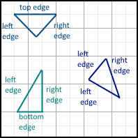
The concepts of left, right, upper and lower faces require clarification. So far, we will not give exact definitions (we will do this when we get to traversal algorithms), but will describe them in a simpler language:
Examples:
Now consider the case of adjacent polygons. If the face is adjacent and is left in one polygon, then the same face is right for all polygons that share this face with this polygon. A similar rule works for the upper and lower faces:

We can use this property to determine which of the adjacent polygons a pixel belongs to. If we agree that a pixel whose center lies on a common face belongs only to polygons for which this face is left, then it will not automatically belong to adjacent polygons, since for them this face is right. And the same for the upper bound.
Despite the fact that the rule of the upper and left faces is found most often, we can use any suitable combination. For example, the rule of the bottom and left sides, top and right, etc. Direct3D requires the use of a top-left rule, OpenGL is not so strict and allows you to use any rule that solves the problem of pixel ownership. I will continue to assume the use of a top-left rule.
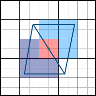
Consider the following two polygons: The
second polygon can be obtained from the first as a result of rotation at a certain angle. As a result, some pixels are additionally included in the final image (such pixels are marked in green), and some, on the contrary, disappear from it (marked in red). Accordingly, we need to take into account the fractional parts of the vertex coordinates. If we discard them, we will get problems when drawing a non-static scene. If, for example, the polygon is made to rotate very slowly, then it will do it jerkingly - since the edges will “jump” sharply from one position to another, instead of correctly processing intermediate results. The difference is easy to understand by comparing these two videos:
Of course, in the case of a static scene, such problems will not arise.
Before proceeding directly to the rasterization algorithms, let us dwell on the interpolation of attributes.
An attribute is some information associated with an object, which is necessary for its correct rendering according to a given algorithm. Anything can be such an attribute. One of the most common options are: color, texture coordinates, normal coordinates. Attribute values are set at the vertices of the object grid. When rasterizing polygons, these attributes are interpolated along the surface of the triangles and are used to calculate the color of each of the pixels.
The simplest example (and a kind of analogue of “hello world”) is the drawing of a triangle, at each vertex of which one attribute is set - color:
In this case, if we assign a color to each pixel of the polygon that is the result of linear interpolation of the colors of the three vertices, we get the following image:
The way the interpolation is done depends on the data that we operate in the rendering process, and they, in turn, depend on the algorithm used in the rasterization. For example, when using the “standard” algorithm, we can use simple linear interpolation of values between two pixels, and when using traversal-algorithms - barycentric coordinates. Therefore, we postpone it until the description of the algorithms themselves.
However, there is still an important topic that needs to be addressed in advance: attribute interpolation with perspective correction.
The simplest interpolation method is linear interpolation in the screen space: after the polygon has been projected onto the projection plane, we linearly interpolate the attributes along the surface of the triangle. It is important to understand that this interpolation is not correct, since it does not take into account the projection performed.
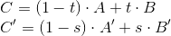
Consider projecting a line onto the projection plane d = 1 . At the starting and ending peaks, certain attributes are set that linearly change in the camera space (and in the world). After the projection is made, these attributes do not grow linearly in the screen space. If, for example, we take the midpoint in the camera space ( v = v0 * 0.5 + v1 * 0.5 ), then after the projection this point will not lie in the middle of the projected line:

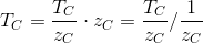
This is most easily noticed when texturing objects (I will use simple texturing without filtering in the examples below). I have not described the texturing process in detail (and this is the topic of a separate article), so for now I will limit myself to a brief description.
When texturing, the attribute of texture coordinates is set at each vertex of the polygon (it is often called uv by the name of the corresponding axes). These are normalized coordinates (from 0 to 1 ) that determine which part of the texture will be used.
Now imagine that we want to draw a textured rectangle and set the four values of the uv attribute so that the whole texture is used:

Everything seems to be fine:
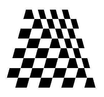
True, this model is located parallel to the projection plane, and therefore there should be no distortions due to the perspective. Let's try to shift the top two vertices by one along the z axis , and the problem will become visible immediately:
Thus, it is necessary to consider the perspective when interpolating the attributes. The key fact to this is that, although z cannot be correctly interpolated in the screen space, 1 / z can. Again, consider the projection of the line:
We also already know that by similar triangles:

Interpolating x in the screen space, we get:

Interpolating x in the camera space, we get:

These three equalities are key and on their basis all subsequent formulas are derived. I will not give a full conclusion, since this is easy to do on my own, and I will describe it only briefly, focusing on the results.
Substituting these two equalities into the equation obtained from the aspect ratios of the triangle, and simplifying all the expressions, we finally get that the reciprocal of the z- coordinate can be linearly interpolated in the screen space:
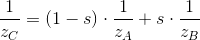
It is important that in this expression the interpolation occurs between the quantities, inverse z- coordinates in the camera space.
Further, suppose that values of a certain attribute are given at the vertices A and B , we denote them by T1 andT2 , which can also be linearly interpolated in the camera space:

Using the intermediate results from the output above, we can write that the value Tc / Zc can also be correctly interpolated in the screen space:

Summing up, we get that 1 / Zc and Tc / Zc can be linearly interpolated in the screen space. Now we can easily get the value of Tc :
Actually, the cost of prospectively correct interpolation lies mainly in this division. If it is not very necessary, it is best to minimize the number of attributes for which it is used and dispense with simple linear interpolation in the screen space, if possible. The correct texturing result is shown below:
To implement perspective correction, we need values that are inverse to the depth ( z- coordinate) of the vertices in the camera space. Recall what happens when multiplied by the projection matrix:

The vertices from the camera space go into the clipping space. In particular, the z- coordinate undergoes certain changes (which will be needed in the future for the depth buffer) and no longer coincides with z- the coordinate vertex in the camera space, so we cannot use it. And what coincides is the w- coordinate, since we explicitly put z from the camera space in it (just look at the 4th column of the matrix). In fact, we need not even z itself , but 1 / z . And we actually get it “for free,” because when we switch to NDC, we divide all the vertices by z (which lies in the w-coordinate):
And that means we can just replace it with the opposite value:
Below we will describe three approaches to polygon rasterization. Full code examples will be missing, since so much of it depends on the implementation, and this will be more confusing than helping. At the end of the article there will be a link to the project, and, if necessary, you can see the implementation code in it.
I called this algorithm “standard” because it is the most commonly described rasterization algorithm for software renderers. It is easier to understand than traversal algorithms and rasterization in uniform coordinates, and, accordingly, easier to implement.
So, let's start with the triangle that we want to rasterize. Assume, for starters, that this is a triangle with a horizontal bottom face.
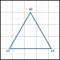
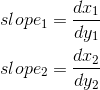
The essence of this algorithm is the sequential movement along the side faces and filling in pixels between them. To do this, first offset values along the X axis are calculated for each offset per unit along the Y axis.
Then, movement along the sides begins. It is important that the movement starts from the nearest center, and not from the Y- coordinate of the vertex v0, since the pixels are represented by these points. If the Y- coordinate v0 already lies on the center, then we still move to the next center on this axis, since v0 lies on both the left and right faces, which means this pixel should not be included in the image:
When we go to the next line , we also start moving only from the next center along the X axis. If the face passes through the center of the pixel, then we include the pixel in the image on the left side, but not on the right.
Similarly, the algorithm works for triangles with a horizontal top side. Those triangles that have no horizontal sides are simply divided into two triangles - one with a horizontal top and one with a horizontal bottom. To do this, look for the intersection of the horizontal line passing through one of the vertices of the triangle ( Y- coordinate average ) with the other face:

After that, each of these triangles is rasterized according to the algorithm above. It is also necessary to correctly calculate the values of z and w coordinates at the new vertex - for example, interpolate them. Similarly, the presence of this vertex must be considered when interpolating attributes.
Attributes are interpolated without perspective correction as follows - when moving along the side faces, we calculate the interpolated attribute values at the start and end points of the line that we are going to rasterize. Then, these values are linearly interpolated along this line. If perspective correction is needed for the attribute, then instead we interpolate T / z along the faces of the polygon (instead of just interpolating simply T is the attribute value), as well as 1 / z . Then, these values at the start and end points of the line are interpolated along it and are used to get the final attribute value taking into account the perspective, according to the formula given above. It must be remembered that 1 / z, to which I refer, actually lies in the w-coordinate of the vector after all the transformations made.
This is a whole group of algorithms that use the same approach based on the equations of the faces of a polygon.
The equation of a face is the equation of the line on which that face lies. In other words, this is the equation of a line passing through two vertices of a polygon. Accordingly, each triangle is characterized by three linear equations:

To begin with, we describe the equation of a line passing through two points (they are the pair of vertices of the triangle):

We can rewrite it in the following form:


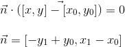
It can be seen from the last expression that the vector n is perpendicular to the vector v0 - v1 (the coordinates are interchanged, and the X-coordinate is taken with a minus sign). Thus, n is the normal to the line formed by two vertices. This is all the same equation of a line, and, therefore, substituting the point (x, y) there and getting zero, we know that this point lies on the line. What about the rest of the values? This is where the normal recording form comes in handy. We know that the scalar product of two vectors calculates the length of the projection of the first vector onto the second, multiplied by the length of the second vector. Normal acts as the first vector, and vector from the first vertex to the point (x, y) acts as the second one:

And we have three possible options:
They are all depicted below:
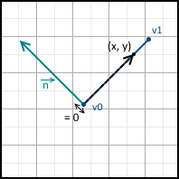
We can also set the equation of the line so that the normal points in the opposite direction - just multiply it by minus one. In the future, I will assume that the equation is designed in such a way that the normal points inside the triangle.
Using these equations, we can define a triangle as the intersection of three positive half-planes.
Thus, the general part of traversal algorithms is as follows:
Let us dwell on the implementation of the top-left rule. Now that we are operating on the normal to the face, we can give more rigorous definitions for the left and top faces:
It is also important to note that the normal coordinates coincide with the coefficients a and b in the canonical equation of the line: ax + by + c = 0 .
Below is an example of a function that determines whether a pixel is in a positive half-plane relative to one of the faces (using the top-left rule). It is enough for her to take three arguments at the input: the value of the equation of the face at the point, and the coordinates of the normal:
A simple and useful optimization when calculating the values of equations: if we know the value in a pixel with coordinates (x, y) , then to calculate the value at the point (x + 1, y) it is enough to add the value of the coefficient a . Similarly, to calculate the value in (x, y + 1), it suffices to add the coefficient b :
The next step is to interpolate the attributes and correct the perspective. For this, barycentric coordinates are used. These are coordinates in which a triangle point is described as a linear combination of vertices (formally, implying that the point is the center of mass of the triangle, with the corresponding vertex weight). We will use the normalized version - i.e. the total weight of the three vertices is equal to one:
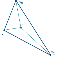
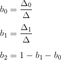
This coordinate system also has a very useful property that allows them to be calculated: barycentric coordinates are equal to the ratio of the area of the triangles formed in the figure above to the total area of the triangle (for this reason they are also sometimes called areal coordinates):
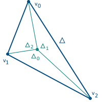
The third coordinate may not be calculated through the area of the triangles, since the sum of the three coordinates is equal to unity - in fact, we have only two degrees of freedom.
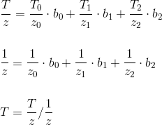
Now everything is ready for linear interpolation of attributes: the attribute value at a given point in the triangle is equal to a linear combination of barycentric coordinates and attribute values at the corresponding vertices:

To correct the perspective, we use a different formula - first, we calculate the interpolated value T / z, then the interpolated value 1 / z , and then divide them into each other to get the final value of T , taking into account the perspective:
The difference between the various traversal algorithms is how the pixels are selected for verification. We will consider several options.
As the name implies, this algorithm simply builds the axis-aligned bounding box of the polygon, and passes through all the pixels inside it. Example:
This algorithm consists of the following steps:
This can be represented as follows:
Check that the pixel is to the left of the polygon as follows - for at least one face whose normal points to the right (i.e. a> 0), the value of the equation of this face is negative.
This algorithm can be considered as an improved version of the backtracking algorithm. Instead of “idling” to go through the pixels in a line until there is a pixel from which we can start moving to the right, we remember information about the pixel from which we started moving on the line, and then go through the pixels to the left and right of him.
This algorithm was originally described in the publication Triangle scan conversion using 2D homogeneous coordinates, Marc Olano & Trey Greer . Its main advantages are the absence of the need for clipping and division by the w-coordinate during the transformation of vertices (with the exception of a couple of reservations - they will be described later).
First of all, suppose that, at the beginning of the rasterization, the x and y coordinates of the vertices contain values that are displayed in the coordinates on the screen by simply dividing by the corresponding w-coordinate. This can slightly change the vertex transformation code, provided that several rasterization algorithms are supported, since it does not include division by w-coordinate. Coordinates in a homogeneous two-dimensional space are transferred directly to a function that performs rasterization.
Let us consider in more detail the question of linear interpolation of attributes along the polygon. Since the value of the attribute (let's call it p ) grows linearly, it must satisfy the following equation (in three-dimensional space):

Since the point (x, y, z) is projected onto the plane using uniform coordinates (x, y, w) , where w = z , we can also write this equation in homogeneous coordinates:

Imagine that we know the coefficients a , b, and c (we will consider finding them a bit later). During rasterization, we are dealing with the coordinates of pixels in the screen space, which are related to the coordinates in a homogeneous space according to the following formula (this was our initial assumption):

We can express the p / w value using only the coordinates in the screen space, by dividing by w:

For getting the correct p value using screen coordinates, we just need to divide this value by 1 / w (or, which is the same thing, multiply by w ):

1 / w, in turn, can be calculated using a similar algorithm - it is enough to imagine that we have a certain parameter that is the same at all vertices: p = [1 1 1] .
Now consider how we can find the coefficients a , b, and c . Since for each attribute its values are set at the vertices of the polygon, we actually have a system of equations of the form:

We can rewrite this system in matrix form:
And the solution:

It is important to note that we need to calculate only one inverse matrix per polygon - then these coefficients can be used to find the correct attribute value at any point on the screen. Also, since we need to calculate the determinant of the matrix to invert it, we get some auxiliary information, since the determinant also calculates the volume of the tetrahedron with vertices at the origin and points of the polygon multiplied by two (this follows from the definition of a mixed product of vectors) If the determinant is equal to zero, this means that the polygon cannot be drawn, because it is either degenerate or rotated by an edge with respect to the camera. Also, the volume of a tetrahedron can be with a plus sign and with a minus sign - and this can be used when cutting off polygons that are turned “back” to the camera (the so-called backface culling). If we consider it correct to order the vertices counterclockwise, then polygons for which the value of the determinant is positive should be skipped (subject to the use of a left-handed coordinate system).
Thus, the issue of attribute interpolation has already been solved - we can calculate the correct value (taking into account the perspective) of any attribute at a given point on the screen. It remains only to decide which points on the screen the polygon belongs to.
Recall how the pixel affiliation to the polygon was verified in traversal algorithms. We calculated the equations of the faces, and then checked their values at the desired point on the screen. If they were all positive (or zero, but belonged to the left or top faces), then we painted over the pixel. Since we already know how to interpolate attributes along the surface of a triangle, we can use the exact same approach, assuming that we interpolate some pseudo-attribute that is equal to zero along the face and some positive value (the most convenient is 1) at the opposite vertex (in fact, this is a plane passing through these faces):

Accordingly, the values of these pseudo-attributes for each of the faces:
Using them, we can calculate the corresponding coefficients a , band with for each of the faces and get their equations:

Now we can similarly interpolate their values along the surface of the triangle and calculate their values at the point we need. If it is positive, or if it is zero, but we are on the left and top faces, the pixel is inside the polygon and must be filled over. We can also apply a small optimization - we do not need exact values of the equations of the faces at all, just its sign is enough. Therefore, dividing by 1 / w can be avoided , we can just check the signs p / w and 1 / w - they must coincide.
Since we operate on the same face equations, much of what was said in the section on traversal algorithms can be applied to this algorithm as well. For example, a top-left rule can be implemented in a similar way, and the values of the equations of faces can be calculated incrementally, which is a useful optimization.
When introducing this algorithm, I wrote that this algorithm does not require clipping, because it operates in uniform coordinates. This is almost entirely true, with the exception of one case. There may be situations when working with w-coordinates of points that are close to the origin (or coincide with it). In this case, overflows may occur during attribute interpolation. So it’s a good idea to add another “face” that is parallel to the xy planeand is located at a distance z near from the origin to avoid such errors.
When describing traversal algorithms, I mentioned several options for choosing a set of pixels that should be checked for a triangle (axis aligned bounding box, backtracking, zigzag algorithms). They can be applied here. This is the situation in which, nevertheless, it will be necessary to divide the vertices by the w-coordinate to calculate boundary values (for example, the coordinates of a bounding box), you should only consider situations when w <= 0 . Of course, there are other ways. Passing through all the pixels of the screen is obviously unsuccessful in view of performance. You can also use tile rasterization, a description of which is beyond the scope of this article.
A project where you can see examples of implementations: github.com/loreglean/lantern . Pull requests with fixes and other things are welcome, it is better to write about errors in the code or questions about it in PM.
Our input is a set of polygons (we will only consider triangles): the coordinates of their vertices (the coordinate system depends on the algorithm) and the attribute values at each of these vertices, which will be further interpolated along the surface of the triangle. There are several pitfalls that I will cover in this article:
- Pixel Filling Rule
- Accuracy
- Perspective correction during attribute interpolation (perspective-correct interpolation)
I will consider three approaches to rasterization:
- "Standard" algorithm using face tilt
- a number of algorithms based on the use of equations of the faces of the polygon (traversal-algorithms)
- uniform rasterization algorithm
Also at the end there will be a link to the project, which is an example of implementation, from there will also be code examples.
The basics
So, rasterization is the process of finding pixels that are “included” in a given polygon. To begin with, we will assume that it is enough for us to fill the polygon with a solid color - nothing more.
Imagine that we have the following triangle for displaying on the screen (all coordinates are already presented in the screen space):
What pixels need to be painted over? A pixel can be entirely outside the polygon, partially in the polygon and entirely in the polygon:
Everything is simple for two cases:
- The pixel is not included in the whole polygon (red color in the picture) - do not paint over
- The pixel is included in the entire polygon (green color in the picture) - paint over
The third case (the pixel is partially inside the polygon) is more complicated. The first decision that comes to mind is to assume that all such pixels are either included in the polygon or not. But it leads to the wrong result. The three-dimensional models that we are going to draw consist of many triangles, which, in general, should not overlap each other. Triangles overlapping each other do not make sense, since they only duplicate existing information. Thus, many polygons have common faces. The simplest example is a rectangle:
Pixels that partially fit into both polygons are marked in orange. Now imagine that we will rasterize both of these polygons. If we decide that all the pixels partially included in the polygon should be filled, we will get the same pixels twice (or more if there is a common vertex for more than two polygons). This may not seem like a problem at first glance, but in fact, it will lead to various artifacts when using some techniques, such as alpha blending (rendering using the alpha channel to simulate transparency). This also leads to a decrease in productivity, because the number of pixels for which we need to calculate attribute values is increasing. If, on the contrary, we decide that such pixels are not included in the final image and should not be filled,
Thus, we came to the understanding that each pixel when filling adjacent polygons must be filled exactly once. This is a requirement that both Direct3D and OpenGL comply with.
The problem arises from the need to display from continuous (screen coordinate system) to discrete (pixels on the monitor). The traditional rasterization algorithm (when rendering without smoothing) solves this as follows: each pixel is associated with a certain point (sample point), which is responsible for the pixel entering the polygon. Also, it is at this point that the values of all necessary attributes are considered. In other words, all the space occupied by a pixel in the coordinate system of the screen is "represented" by one point. As a rule, this is the center: (0.5, 0.5):
Theoretically, you can take any point inside the pixel, instead of the center. Other values will lead to the fact that the image can be "shifted" by a pixel in one direction. Also, in the situation with adjacent polygons, for pixels in which the vertices of the triangles are not located, the use of a point (0.5, 0.5) has a good property: this point is included in the polygon that covers more than 50% of the area of the rectangle representing the pixel.
Thus, if the center of the pixel is included in the polygon, then it is considered that the pixel belongs to the polygon. But now the following problem arises: what if two polygons have a common face that passes through the center of the pixel? We already realized that a pixel should belong to only one of the two triangles, but which one? In the picture below, such a pixel is marked in red:
This problem is solved by the so-called “filling convention”.
Filling Agreement
So, suppose we are faced with the situation described above - two polygons share a face that passes exactly through the center of the pixel. Our task is to find out which of the polygons this pixel belongs to.
The de facto standard is the so-called top-left rule: it follows DirectX and most OpenGL implementations. The essence of this rule is this: if the face of the polygon passes through the center of the pixel, then this pixel belongs to the polygon in two cases - if it is the left side or the top face (hence the name).
The concepts of left, right, upper and lower faces require clarification. So far, we will not give exact definitions (we will do this when we get to traversal algorithms), but will describe them in a simpler language:
- The top face is the horizontal face that is above all other faces
- Bottom - a horizontal face that is below all other faces
- Left side - a face that is located on the left side of the triangle and is not horizontal
- The right side is the face that is located on the right side of the triangle and is not horizontal
Examples:
Now consider the case of adjacent polygons. If the face is adjacent and is left in one polygon, then the same face is right for all polygons that share this face with this polygon. A similar rule works for the upper and lower faces:
We can use this property to determine which of the adjacent polygons a pixel belongs to. If we agree that a pixel whose center lies on a common face belongs only to polygons for which this face is left, then it will not automatically belong to adjacent polygons, since for them this face is right. And the same for the upper bound.
Despite the fact that the rule of the upper and left faces is found most often, we can use any suitable combination. For example, the rule of the bottom and left sides, top and right, etc. Direct3D requires the use of a top-left rule, OpenGL is not so strict and allows you to use any rule that solves the problem of pixel ownership. I will continue to assume the use of a top-left rule.
Accuracy
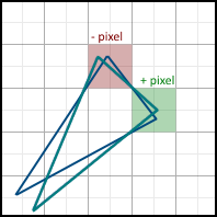
Consider the following two polygons: The
second polygon can be obtained from the first as a result of rotation at a certain angle. As a result, some pixels are additionally included in the final image (such pixels are marked in green), and some, on the contrary, disappear from it (marked in red). Accordingly, we need to take into account the fractional parts of the vertex coordinates. If we discard them, we will get problems when drawing a non-static scene. If, for example, the polygon is made to rotate very slowly, then it will do it jerkingly - since the edges will “jump” sharply from one position to another, instead of correctly processing intermediate results. The difference is easy to understand by comparing these two videos:
Of course, in the case of a static scene, such problems will not arise.
Attribute Interpolation
Before proceeding directly to the rasterization algorithms, let us dwell on the interpolation of attributes.
An attribute is some information associated with an object, which is necessary for its correct rendering according to a given algorithm. Anything can be such an attribute. One of the most common options are: color, texture coordinates, normal coordinates. Attribute values are set at the vertices of the object grid. When rasterizing polygons, these attributes are interpolated along the surface of the triangles and are used to calculate the color of each of the pixels.
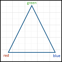
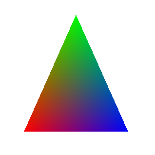
The simplest example (and a kind of analogue of “hello world”) is the drawing of a triangle, at each vertex of which one attribute is set - color:
In this case, if we assign a color to each pixel of the polygon that is the result of linear interpolation of the colors of the three vertices, we get the following image:
The way the interpolation is done depends on the data that we operate in the rendering process, and they, in turn, depend on the algorithm used in the rasterization. For example, when using the “standard” algorithm, we can use simple linear interpolation of values between two pixels, and when using traversal-algorithms - barycentric coordinates. Therefore, we postpone it until the description of the algorithms themselves.
However, there is still an important topic that needs to be addressed in advance: attribute interpolation with perspective correction.
The simplest interpolation method is linear interpolation in the screen space: after the polygon has been projected onto the projection plane, we linearly interpolate the attributes along the surface of the triangle. It is important to understand that this interpolation is not correct, since it does not take into account the projection performed.
Consider projecting a line onto the projection plane d = 1 . At the starting and ending peaks, certain attributes are set that linearly change in the camera space (and in the world). After the projection is made, these attributes do not grow linearly in the screen space. If, for example, we take the midpoint in the camera space ( v = v0 * 0.5 + v1 * 0.5 ), then after the projection this point will not lie in the middle of the projected line:
This is most easily noticed when texturing objects (I will use simple texturing without filtering in the examples below). I have not described the texturing process in detail (and this is the topic of a separate article), so for now I will limit myself to a brief description.
When texturing, the attribute of texture coordinates is set at each vertex of the polygon (it is often called uv by the name of the corresponding axes). These are normalized coordinates (from 0 to 1 ) that determine which part of the texture will be used.
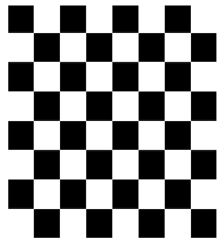
Now imagine that we want to draw a textured rectangle and set the four values of the uv attribute so that the whole texture is used:
Everything seems to be fine:
True, this model is located parallel to the projection plane, and therefore there should be no distortions due to the perspective. Let's try to shift the top two vertices by one along the z axis , and the problem will become visible immediately:
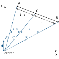
Thus, it is necessary to consider the perspective when interpolating the attributes. The key fact to this is that, although z cannot be correctly interpolated in the screen space, 1 / z can. Again, consider the projection of the line:
We also already know that by similar triangles:
Interpolating x in the screen space, we get:
Interpolating x in the camera space, we get:
These three equalities are key and on their basis all subsequent formulas are derived. I will not give a full conclusion, since this is easy to do on my own, and I will describe it only briefly, focusing on the results.
Substituting these two equalities into the equation obtained from the aspect ratios of the triangle, and simplifying all the expressions, we finally get that the reciprocal of the z- coordinate can be linearly interpolated in the screen space:
It is important that in this expression the interpolation occurs between the quantities, inverse z- coordinates in the camera space.
Further, suppose that values of a certain attribute are given at the vertices A and B , we denote them by T1 andT2 , which can also be linearly interpolated in the camera space:
Using the intermediate results from the output above, we can write that the value Tc / Zc can also be correctly interpolated in the screen space:
Summing up, we get that 1 / Zc and Tc / Zc can be linearly interpolated in the screen space. Now we can easily get the value of Tc :
Actually, the cost of prospectively correct interpolation lies mainly in this division. If it is not very necessary, it is best to minimize the number of attributes for which it is used and dispense with simple linear interpolation in the screen space, if possible. The correct texturing result is shown below:
To implement perspective correction, we need values that are inverse to the depth ( z- coordinate) of the vertices in the camera space. Recall what happens when multiplied by the projection matrix:
The vertices from the camera space go into the clipping space. In particular, the z- coordinate undergoes certain changes (which will be needed in the future for the depth buffer) and no longer coincides with z- the coordinate vertex in the camera space, so we cannot use it. And what coincides is the w- coordinate, since we explicitly put z from the camera space in it (just look at the 4th column of the matrix). In fact, we need not even z itself , but 1 / z . And we actually get it “for free,” because when we switch to NDC, we divide all the vertices by z (which lies in the w-coordinate):
float const w_inversed{ 1.0f / v.w };
v.x *= w_inversed;
v.y *= w_inversed;
v.z *= w_inversed;
// NDC to screen
// ...
And that means we can just replace it with the opposite value:
float const w_inversed{ 1.0f / v.w };
v.x *= w_inversed;
v.y *= w_inversed;
v.z *= w_inversed;
v.w = w_inversed;
// NDC to screen
// ...
Rasterization Algorithms
Below we will describe three approaches to polygon rasterization. Full code examples will be missing, since so much of it depends on the implementation, and this will be more confusing than helping. At the end of the article there will be a link to the project, and, if necessary, you can see the implementation code in it.
"Standard" algorithm
I called this algorithm “standard” because it is the most commonly described rasterization algorithm for software renderers. It is easier to understand than traversal algorithms and rasterization in uniform coordinates, and, accordingly, easier to implement.
So, let's start with the triangle that we want to rasterize. Assume, for starters, that this is a triangle with a horizontal bottom face.
The essence of this algorithm is the sequential movement along the side faces and filling in pixels between them. To do this, first offset values along the X axis are calculated for each offset per unit along the Y axis.
Then, movement along the sides begins. It is important that the movement starts from the nearest center, and not from the Y- coordinate of the vertex v0, since the pixels are represented by these points. If the Y- coordinate v0 already lies on the center, then we still move to the next center on this axis, since v0 lies on both the left and right faces, which means this pixel should not be included in the image:
When we go to the next line , we also start moving only from the next center along the X axis. If the face passes through the center of the pixel, then we include the pixel in the image on the left side, but not on the right.
Similarly, the algorithm works for triangles with a horizontal top side. Those triangles that have no horizontal sides are simply divided into two triangles - one with a horizontal top and one with a horizontal bottom. To do this, look for the intersection of the horizontal line passing through one of the vertices of the triangle ( Y- coordinate average ) with the other face:
After that, each of these triangles is rasterized according to the algorithm above. It is also necessary to correctly calculate the values of z and w coordinates at the new vertex - for example, interpolate them. Similarly, the presence of this vertex must be considered when interpolating attributes.
Attributes are interpolated without perspective correction as follows - when moving along the side faces, we calculate the interpolated attribute values at the start and end points of the line that we are going to rasterize. Then, these values are linearly interpolated along this line. If perspective correction is needed for the attribute, then instead we interpolate T / z along the faces of the polygon (instead of just interpolating simply T is the attribute value), as well as 1 / z . Then, these values at the start and end points of the line are interpolated along it and are used to get the final attribute value taking into account the perspective, according to the formula given above. It must be remembered that 1 / z, to which I refer, actually lies in the w-coordinate of the vector after all the transformations made.
Traversal algorithms
This is a whole group of algorithms that use the same approach based on the equations of the faces of a polygon.
The equation of a face is the equation of the line on which that face lies. In other words, this is the equation of a line passing through two vertices of a polygon. Accordingly, each triangle is characterized by three linear equations:
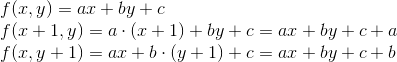
To begin with, we describe the equation of a line passing through two points (they are the pair of vertices of the triangle):
We can rewrite it in the following form:
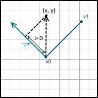
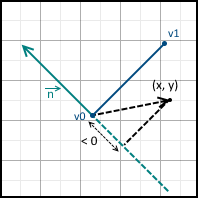
It can be seen from the last expression that the vector n is perpendicular to the vector v0 - v1 (the coordinates are interchanged, and the X-coordinate is taken with a minus sign). Thus, n is the normal to the line formed by two vertices. This is all the same equation of a line, and, therefore, substituting the point (x, y) there and getting zero, we know that this point lies on the line. What about the rest of the values? This is where the normal recording form comes in handy. We know that the scalar product of two vectors calculates the length of the projection of the first vector onto the second, multiplied by the length of the second vector. Normal acts as the first vector, and vector from the first vertex to the point (x, y) acts as the second one:
And we have three possible options:
- The value is 0 - the point lies on a straight line.
- Value greater than 0 - point lies in the positive half-plane
- Value less than 0 - the point lies in the negative half-plane
They are all depicted below:
We can also set the equation of the line so that the normal points in the opposite direction - just multiply it by minus one. In the future, I will assume that the equation is designed in such a way that the normal points inside the triangle.
Using these equations, we can define a triangle as the intersection of three positive half-planes.
Thus, the general part of traversal algorithms is as follows:
- We calculate the values of the equations of the faces for the point
- If all values are positive, the pixel is painted over. If one of them is zero, then the pixel lies on one of the faces, and we use the top-left rule to decide whether the pixel belongs to the polygon
- Go to the next pixel
Let us dwell on the implementation of the top-left rule. Now that we are operating on the normal to the face, we can give more rigorous definitions for the left and top faces:
- The left side is the face whose normal has a positive x-coordinate (i.e., points to the right)
- The upper face is the face whose normal has a negative y-coordinate, if the Y axis points up. If the Y axis points down (I will stick to this option), then the y-coordinate of the upper faces is positive
It is also important to note that the normal coordinates coincide with the coefficients a and b in the canonical equation of the line: ax + by + c = 0 .
Below is an example of a function that determines whether a pixel is in a positive half-plane relative to one of the faces (using the top-left rule). It is enough for her to take three arguments at the input: the value of the equation of the face at the point, and the coordinates of the normal:
Code example
inline bool pipeline::is_point_on_positive_halfplane_top_left(
	float const edge_equation_value, float const edge_equation_a, float const edge_equation_b) const
{
	// Если точка находится на грани, используем top-left rule
	//
	if (std::abs(edge_equation_value) < EPSILON)
	{
		if (std::abs(edge_equation_a) < EPSILON)
		{
			// edge.a == 0.0f, значит это горизонтальная грань, либо верхняя, либо нижняя
			//
			// Если y-координата нормали положительна, мы на верхней грани
			// Иначе на нижней
			return edge_equation_b > 0.0f;
		}
		else
		{
			// Если x-координата нормали положительна, мы на левой грани
			// Иначе на правой
			return edge_equation_a > 0.0f;
		}
	}
	else
	{
		// Просто проверяем, что мы в положительной полуплоскости
		return edge_equation_value > 0.0f;
	}
}
A simple and useful optimization when calculating the values of equations: if we know the value in a pixel with coordinates (x, y) , then to calculate the value at the point (x + 1, y) it is enough to add the value of the coefficient a . Similarly, to calculate the value in (x, y + 1), it suffices to add the coefficient b :
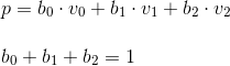
The next step is to interpolate the attributes and correct the perspective. For this, barycentric coordinates are used. These are coordinates in which a triangle point is described as a linear combination of vertices (formally, implying that the point is the center of mass of the triangle, with the corresponding vertex weight). We will use the normalized version - i.e. the total weight of the three vertices is equal to one:
This coordinate system also has a very useful property that allows them to be calculated: barycentric coordinates are equal to the ratio of the area of the triangles formed in the figure above to the total area of the triangle (for this reason they are also sometimes called areal coordinates):
The third coordinate may not be calculated through the area of the triangles, since the sum of the three coordinates is equal to unity - in fact, we have only two degrees of freedom.
Now everything is ready for linear interpolation of attributes: the attribute value at a given point in the triangle is equal to a linear combination of barycentric coordinates and attribute values at the corresponding vertices:
To correct the perspective, we use a different formula - first, we calculate the interpolated value T / z, then the interpolated value 1 / z , and then divide them into each other to get the final value of T , taking into account the perspective:
The difference between the various traversal algorithms is how the pixels are selected for verification. We will consider several options.
AABB algorithm
As the name implies, this algorithm simply builds the axis-aligned bounding box of the polygon, and passes through all the pixels inside it. Example:
Backtracking algorithm
This algorithm consists of the following steps:
- Start at the topmost pixel below the topmost vertex
- We move to the left until we meet a pixel to the left of the polygon (backtracking)
- Move to the right and paint the pixels until we meet a pixel to the right of the polygon
- Go to the line below and start again from the second step.
This can be represented as follows:
Check that the pixel is to the left of the polygon as follows - for at least one face whose normal points to the right (i.e. a> 0), the value of the equation of this face is negative.
Zigzag algorithm
This algorithm can be considered as an improved version of the backtracking algorithm. Instead of “idling” to go through the pixels in a line until there is a pixel from which we can start moving to the right, we remember information about the pixel from which we started moving on the line, and then go through the pixels to the left and right of him.
- Start at the topmost pixel below the topmost vertex
- Remember the position
- We move to the left and paint over the pixels entering the polygon until we meet a pixel to the left of the polygon (backtracking)
- Возвращаемся к пикселю, с которого мы начали (мы запомнили его в шаге 2), и двигаемся направо, закрашивая пиксели, входящие в полигон, пока не встретим пиксель вне полигона
- Переходим на линию ниже и начинаем снова со второго шага
Алгоритм растеризации в однородных координатах
This algorithm was originally described in the publication Triangle scan conversion using 2D homogeneous coordinates, Marc Olano & Trey Greer . Its main advantages are the absence of the need for clipping and division by the w-coordinate during the transformation of vertices (with the exception of a couple of reservations - they will be described later).
First of all, suppose that, at the beginning of the rasterization, the x and y coordinates of the vertices contain values that are displayed in the coordinates on the screen by simply dividing by the corresponding w-coordinate. This can slightly change the vertex transformation code, provided that several rasterization algorithms are supported, since it does not include division by w-coordinate. Coordinates in a homogeneous two-dimensional space are transferred directly to a function that performs rasterization.
Let us consider in more detail the question of linear interpolation of attributes along the polygon. Since the value of the attribute (let's call it p ) grows linearly, it must satisfy the following equation (in three-dimensional space):
Since the point (x, y, z) is projected onto the plane using uniform coordinates (x, y, w) , where w = z , we can also write this equation in homogeneous coordinates:
Imagine that we know the coefficients a , b, and c (we will consider finding them a bit later). During rasterization, we are dealing with the coordinates of pixels in the screen space, which are related to the coordinates in a homogeneous space according to the following formula (this was our initial assumption):
We can express the p / w value using only the coordinates in the screen space, by dividing by w:
For getting the correct p value using screen coordinates, we just need to divide this value by 1 / w (or, which is the same thing, multiply by w ):
1 / w, in turn, can be calculated using a similar algorithm - it is enough to imagine that we have a certain parameter that is the same at all vertices: p = [1 1 1] .
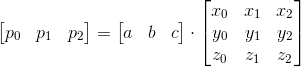
Now consider how we can find the coefficients a , b, and c . Since for each attribute its values are set at the vertices of the polygon, we actually have a system of equations of the form:
We can rewrite this system in matrix form:
And the solution:
It is important to note that we need to calculate only one inverse matrix per polygon - then these coefficients can be used to find the correct attribute value at any point on the screen. Also, since we need to calculate the determinant of the matrix to invert it, we get some auxiliary information, since the determinant also calculates the volume of the tetrahedron with vertices at the origin and points of the polygon multiplied by two (this follows from the definition of a mixed product of vectors) If the determinant is equal to zero, this means that the polygon cannot be drawn, because it is either degenerate or rotated by an edge with respect to the camera. Also, the volume of a tetrahedron can be with a plus sign and with a minus sign - and this can be used when cutting off polygons that are turned “back” to the camera (the so-called backface culling). If we consider it correct to order the vertices counterclockwise, then polygons for which the value of the determinant is positive should be skipped (subject to the use of a left-handed coordinate system).
Thus, the issue of attribute interpolation has already been solved - we can calculate the correct value (taking into account the perspective) of any attribute at a given point on the screen. It remains only to decide which points on the screen the polygon belongs to.
Recall how the pixel affiliation to the polygon was verified in traversal algorithms. We calculated the equations of the faces, and then checked their values at the desired point on the screen. If they were all positive (or zero, but belonged to the left or top faces), then we painted over the pixel. Since we already know how to interpolate attributes along the surface of a triangle, we can use the exact same approach, assuming that we interpolate some pseudo-attribute that is equal to zero along the face and some positive value (the most convenient is 1) at the opposite vertex (in fact, this is a plane passing through these faces):
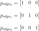
Accordingly, the values of these pseudo-attributes for each of the faces:
Using them, we can calculate the corresponding coefficients a , band with for each of the faces and get their equations:
Now we can similarly interpolate their values along the surface of the triangle and calculate their values at the point we need. If it is positive, or if it is zero, but we are on the left and top faces, the pixel is inside the polygon and must be filled over. We can also apply a small optimization - we do not need exact values of the equations of the faces at all, just its sign is enough. Therefore, dividing by 1 / w can be avoided , we can just check the signs p / w and 1 / w - they must coincide.
Since we operate on the same face equations, much of what was said in the section on traversal algorithms can be applied to this algorithm as well. For example, a top-left rule can be implemented in a similar way, and the values of the equations of faces can be calculated incrementally, which is a useful optimization.
When introducing this algorithm, I wrote that this algorithm does not require clipping, because it operates in uniform coordinates. This is almost entirely true, with the exception of one case. There may be situations when working with w-coordinates of points that are close to the origin (or coincide with it). In this case, overflows may occur during attribute interpolation. So it’s a good idea to add another “face” that is parallel to the xy planeand is located at a distance z near from the origin to avoid such errors.
When describing traversal algorithms, I mentioned several options for choosing a set of pixels that should be checked for a triangle (axis aligned bounding box, backtracking, zigzag algorithms). They can be applied here. This is the situation in which, nevertheless, it will be necessary to divide the vertices by the w-coordinate to calculate boundary values (for example, the coordinates of a bounding box), you should only consider situations when w <= 0 . Of course, there are other ways. Passing through all the pixels of the screen is obviously unsuccessful in view of performance. You can also use tile rasterization, a description of which is beyond the scope of this article.
That's all
A project where you can see examples of implementations: github.com/loreglean/lantern . Pull requests with fixes and other things are welcome, it is better to write about errors in the code or questions about it in PM.