Majwick Filter

Preface from the translator

Here is one of the newest methods for calculating spatial orientation according to the readings of the sensors of the accelerometer, gyroscope and compass - the Majwick filter, which, according to the author, gives a better result than applying a filter based on the Kalman method in results and performance. The author is Sebastian Majwick (his online store ). The method is described in an article in English. This work is protected at the University of Bristol Translation I did not find. The translator of me is so-so, especially such complex texts. But we are interested in what kind of method?

In some places I’ll add on my own - there the text is in italics. I found more than 10 typos in the original text. In general, it was quite difficult, so help is welcome - write in the comments where you need to rephrase, in general, where something is wrong.

Filter of data arrays of inertial and inertial-magnetic sensors to determine the orientation

April 30, 2010

From the author

This article describes a new filter for sensor readings for determining spatial orientation in two versions . The first option is applicable to inertial navigation systems (ANNs), including an accelerometer and a gyroscope. The second option is applicable to ANNs, which include an additional 3-axis magnetometer (the abbreviation MARG stands for “Magnetic, Angular Rate and Gravity” ). The implementation of ANN with a magnetometer involves the compensation of magnetic distortion and compensation of the displacement of the gyroscope. As a tool, quaternions are used, which allow the use of accelerometer and magnetometer data for analytical calculations and optimization using the gradient descent methodin obtaining the error in the direction of the gyroscope in the form of a quaternion derivative. Benefits include:

• low cost of computing resources - 277 simple arithmetic operations each filter update (109 operations without a magnetometer);
• efficiency at low sampling frequencies (e.g. 10 Hz);
• Contains 1 (without magnetometer) or 2 adjustable parameters determined on the observed characteristics of the system.

Accuracy was evaluated empirically using commercially available orientation sensors. Reference orientation values ​​obtained using an optical measurement system. A simple calibration method for using optical measuring equipment is presented in this paper.

Accuracy is also compared to a patented Kalman-based filter for orientation sensors. The results show that this filter reaches a level of accuracy that exceeds the filter based on the Kalman method:
<0.6 degrees standard deviation in a stationary state;
<0.8 degrees standard deviation when moving.
Due to the low computational load and the ability to operate at low sampling frequencies, new possibilities are opening up for the application of ANNs for real-time devices with low computational capabilities and high sampling rate requirements.

1. Introduction

Accurate determination of spatial orientation plays an important role in many areas, including:

• Aerospace [1, 2, 3];
• Robotics [4, 5];
• Navigation [6, 7];
• Analysis of human movements [8, 9]
• The interaction of human and machine movements [10].

While various technologies allow you to measure orientation, inertial sensor systems have the advantage of complete autonomy - the measured object is not limited in movement, not limited to any specific environment or location. Inertial Measurement Unit ( BII, or from the English IMU - Inertial Measurement Unit) consists of gyroscopes and accelerometers that track rotational and translational movements. In order to make 3D measurements, it is required that the axes of the sensors are mutually perpendicular. AGM is a hybrid BII, which includes a triaxial magnetometer. A system without a magnetometer can determine the orientation relative to the direction of gravity, which is sufficient for many applications [4, 2, 8, 1]. Inertial navigation systems use a reporting system known as “heading, pitch, roll” (AHRS - Attitude and Heading Reference Systems) , and are able to provide a complete measurement of orientation relative to gravity and the earth's magnetic field.

The gyroscope measures the angular velocity, which under known initial conditions can be integrated over time to obtain the orientation of the sensor [11, 12]. Accurate gyroscopes such as a ring laser are too expensive and bulky for most applications. On the other hand, less accurate MEMS sensors (Micro Electrical Mechanical System - micromechanical electronic systems) are used in most applications [13]. The integration of measurement errors will lead to the accumulation of errors in the calculation of orientation. Thus, gyroscopes, by themselves, cannot provide an absolute measurement of orientation. The accelerometer and magnetometer measure the gravitational and magnetic fields of our planet, and accordingly can determine the absolute value of orientation in space.

However, they are most likely to be exposed to high noise levels. For example, acceleration due to movement will shift the controlled direction of gravity. The task of the orientation filter is to calculate a single orientation estimate obtained by measuring the accelerometer, gyroscope and magnetometer.

The Kalman filter [14] has become the recognized basis for constructing the majority of orientation determination algorithms [4, 15, 16, 17] and commercial orientation systems and inertial modules:

• xsens [18],
• Microstrain [19],
• VectorNav [20],
• InterSense [21],
• PNI [22],
• Crossbow [23],

- All are based on its use. The widespread use of Kalman solutions is proof of their accuracy and efficiency, however, they have several disadvantages. They can be difficult to implement, as shown in the available literature [3, 4, 15, 16, 17, 24, 25, 26, 27, 28, 29, 30, 31, 32]. Linear regression of iteration, is fundamental for Kalman processes, the requirements for sampling frequency, significantly exceeding the throughput of the object. For example, a sampling frequency between 512 Hz and 30 kHz can be used in motion capture applications . The state of the relation describing the rotating kinematics in three dimensions, as a rule, requires more state vectors and the implementation of the extended Kalman filter [4, 17, 24] to linearize the problem.

These problems require a large computational load to implement Kalman solutions, but also provide clear motives for implementing alternative approaches. Many previous approaches to solving these problems were based either on fuzzy processing [2, 5] or on fixing a filter [33] in favor of an accelerometer for determining orientation at low angular velocities and integrating gyroscope measurements when detecting high angular velocities. This approach is simple, but can only be effective under limited operating conditions. Bachmann and others [34] proposed an alternative approach in which the filter achieves optimal synthesis of measurement data at all angular velocities. However, the process requires least-squares approximation, which also adds computational load. Mahoney and others [35] developed a complimentary filter, which, as practice shows, is an effective and efficient solution. However, accuracy is only suitable for ANNs without a magnetometer.

This article describes a new orientation filter that is applicable to both ANNs without a magnetometer and ANNs with a magnetometer. The filter is engaged in processing data arrays coming from sensors and removes the problems of accuracy and tuning filter parameters based on Kalman's approaches. The filter uses the quaternion to represent the orientation (for example [34, 17, 24, 30, 32]) to describe the position in space in three dimensions and does not contain problems associated with the description of the position by Euler angles (folding frames). The article presents a complete conclusion and empirical estimates of the new filter. Its accuracy is compared with existing industrial filters and tested by an optical measurement system. Innovative aspects of the proposed filter include:

• two adjustable parameters (one for implementation without a magnetometer) determined by the observed characteristics of the system;
• analytical calculations and optimization using the gradient descent method, which increases accuracy at low sampling frequencies;
• compensation of magnetic distortions and compensation of zero bias gyroscope in real time.

2. Quaternions

This section of the article is not so interesting - it describes what a quaternion and some basic operations are. All this can be seen in the article with pictures . It is important for us to pay attention to the notation system used by the author.

Fig. 1. The orientation of the axes B is achieved by rotating the axes A around the axis in the reporting system A by an angle θ.

A quaternion is a four-dimensional complex number that can be used to represent the orientation of a pointed body or coordinates in three-dimensional space. The orientation of the reporting system B with respect to the reporting system A can be described by turning it through an angle θ around the axis in the reporting system A. This is shown in Figure 1, where there are mutually orthogonal unit vectors , anddefined by the main axis of the coordinate systems A and B, respectively. The quaternion describing this orientation is defined by equation (1), where Rx, Ry, and Rz are the components of the vector in the corresponding X, Y, and Z axes of the reporting system A. For naming variables, reporting systems and vectors, the Craig designation system is used for notation and subscript [ 37].

The leading lower index in front denotes the target reporting system, and the upper index standing in front indicates the reporting system relative to which the variable is set. Further in the text, index S denotes the sensor reporting system, and index E denotes the Earth reporting system. For example, describes the orientation of the B axes with respect to the A axes, andrepresents a vector in the reporting system A. Quaternion arithmetic often requires that the quaternion be normalized to unity. Therefore, usually all quaternions describing orientation have a length equal to one.



Please note - in this article, the W component of the quaternion comes first (it is often placed at the end).
Omnidirectional quaternions are indicated by * (asterisk) and are used to change the reporting system. For example, it is anti-directional with respect to * and describes the orientation of the reporting system A with respect to B. The anti-directional vector k is determined by equation (2).



The quaternion resulting from the operation can be used to determine composite orientations (series of turns). For example, for two orientations, and can be found by formula (3).



The result of multiplication for two quaternions a and b can be found using the Hamilton rule and is determined by formula (4). When changing the places of the factors, the result is different (multiplication of quaternions is associative, but not commutative).



The three-dimensional vector can be rotated by a quaternion using the ratio described in equation (5) [36]. and these are vectors in the coordinate system A and B, respectively, where each vector contains 0 as a component of W to make them 4 component vectors (quaternions) .


The orientation described by the quaternion can be described as a rotation matrixdetermined by the formula (6) [36].



The Euler angles ψ, θ and φ in the so-called aerospace sequence [36] describe the orientation of the axes achieved by successive rotations relative to the reporting system A, using the angle ψ around the Z axis, θ around the Y axis, and φ around the X axis. Such Euler angles can be obtained from the quaternion using equations (7), (8) and (9).

3. Filter

3.1. Orientation from angular velocity

A three-axis gyroscope measures the angular velocities ωx, ωy and ωz relative to the X, Y, Z axes, respectively, in the sensor reporting system. If the values ​​of these velocities (rad / sec) are converted into a quaternion by a certain equation (10), then the derivative quaternion describing the speed in the Earth's reporting system with respect to the sensor reporting system can be calculated [38] by equation (11):


The orientation in the global reporting system with respect to the local sensor reporting system at time t can be calculated by numerically integrating the quaternions of derivatives , as described in equations (12) and (13), provided that the initial orientation in space is known.

where is the angular velocity measured by the sensor at time t;
∆t - delay between measurements (sampling period);
- previous result of orientation assessment.
Index ω indicates that the quaternion is calculated from angular velocities.

3.2. Orientation from vector observations

A three-axis accelerometer measures the magnitude and direction of the gravitational field in the local coordinate system along with linear accelerations due to the movement of the sensor. In the same way, a three-axis magnetometer measures the magnitude and direction of the earth’s magnetic field in a local reporting system along with local magnetic distortions. In the context of the orientation filter, it will initially assume that the accelerometer will only measure gravity, the magnetometer will only measure the Earth’s magnetic field (the device should be stationary for some time) .

If the direction of the Earth’s field is known in its coordinate system, then measuring the direction in the sensor coordinate system will allow you to calculate the position of the sensor coordinate system relative to the Earth coordinate system. However, for any such measurement there will not be a single solution, but there will be an infinite number of solutions represented by all those orientations achieved by rotating the orientation around a rotation parallel to the direction of the field (magnetic or gravity) . In some cases, a solution can be represented as Euler angles, where there will be two known angles and one unknown. An unknown angle will rotate around an axis parallel to the direction of the field. A quaternion requires a complete solution. This can be achieved by the optimization task, where the orientation of the sensorthis is what aligns a predetermined field direction in the earth's coordinate system with the measured direction in the sensor coordinate system using the rotation operation defined by equation (5). Therefore, it can be found as a solution to equation (14), where equation (15) determines the objective function. The components of each vector are defined in equations (16), (17) and (18).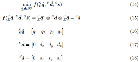

There are many optimization algorithms, but the gradient descent method is one of the simplest to implement and calculate. Equation (19) describes this method for n iterations as a result of orientation estimation based on the “initial approximation” of orientation and step size µ. Equation (20) calculates the gradient of the surface of solutions determined by the objective function and itsJacobian , simplified to the three-component vectors defined in equations (21) and (22), respectively.


Equations (19) - (22) describe the general form of the algorithm applicable to the field, initially oriented in any direction. However, if the direction of the field can be considered only in one or two axes of the global coordinate system, the equation is simplified. The corresponding agreement will assume that the direction of gravity is directed vertically along the Z axis, as shown in equation (23). Substituting the quaternion and normalized measurements of the accelerometer , and respectively into equations (21) and (22), we obtain equation (25) and (26).


The direction of the earth’s magnetic field can also be considered to be located in the same plane and measured in the horizontal and vertical axes. The vertical component depends on the point on the globe at which the measurement takes place. For England, this value is between 65 and 70 degrees relative to the horizon [39]. This can be represented by equation (27). Substituting and normalized measurement values , and respectively in the equations (21) and (22) we obtain the equation (29) and (30).


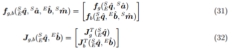
As already discussed, measuring the Earth's gravity or magnetic field alone does not provide a unique sensor orientation. To do this, the measurements and direction ratios of both fields must be combined as described in equations (31) and (32). While the solution surface created by the objective functions in equations (25) and (29) have at least one defined in accordance with the solution surface determined using equation (31), so the minimum is determined at one point, provided that .


The traditional optimization approach will require several iterations of equation (19) to calculate the result for each new orientation and the corresponding sensor measurements. Effective algorithms also require a step size μ to adjust the result at each iteration to the optimal value, usually obtained from the second derivative of the objective function, Hesse. Nevertheless, these requirements significantly increase the computational load of the algorithm and are not necessary in our business. It is acceptable for us to calculate one iteration per time counting, provided that the adjustable convergence rate µt is equal to or greater than the physical rate of orientation change. Equation (33) calculates the approximate direction calculated at time t based on a previous orientation estimateand the objective gradient function ∇f determined by measuring the sensors and at time t. The shape ∇f is selected according to the sensors in use, as shown in equation (34). Index ∇ means that the quaternion is calculated using the gradient descent method.


The optimal value of µt can be defined as one that provides the rate of convergence and is limited by the physical speed of orientation, as this avoids overshooting due to an excessively large step size. Therefore, µt can be calculated using equation (35), where ∆t is the time between measurements, is the physical rate of change of orientation, measured by a gyroscope, α is the increase in µ to take noise into account when measured by an accelerometer and magnetometer.

3.3. Combining Filter Algorithm

We see that the orientation of the sensor with respect to the Earth is obtained by combining the calculations of the orientation of and calculated using equations (13) and (33), respectively. The union and is described by equation (36), where γt and (1 - γt) are the weights applied to each orientation calculation.


The optimal value of γt can be defined as the one at which the weighted divergence is equal to the weighted convergence . This is represented by equation (37), where is the rate of convergence , and β is the rate of divergence , expressed as the value of the quaternion, derived from the corresponding measurement error of the gyroscope. Equation (37) can be modified to determine γt in equation (38).


Equations (36) and (38) provide the optimal combination, and provided that the convergence rate is regulated by α, which is greater than or equal to the physical rate of change of orientation. Therefore, α does not have an upper bound. If we assume that α is very large, then µt is determined by expression (35), and also becomes very large values ​​in the simplified equation of the orientation filter. The large values ​​of µt used in equation (33) mean that it becomes negligible and the equation can be rewritten in the form of expression (39).


Equation (38), which calculates γt, can be further simplified by accepting the insignificance of β in the denominator, and then the expression can be rewritten in the form of equation (40). From equation (40), it is quite possible that γt ≈ 0.


Substituting equations (13), (39) and (40) into equation (36), we obtain directly equation (41). Note that γt in equation (41) is replaced by both expression (39) and 0.


Equation (41) can be simplified to equation (42), where is the calculated rate of change of orientation determined by expression (43); Is the direction of error defined by expression (44).



From equations (42), (43) and (44) we see that the filter calculates the orientation by numerically integrating the calculated orientation speed . The filter calculates as the rate of change in orientation measured by the gyroscope, the same, but with the error of the gyroscope measurement, β is the compensation in the direction of the estimated error;calculated on the basis of measurements of the accelerometer and magnetometer. Fig. 2 shows a block diagram of a complete implementation of an orientation filter for an ANN.


Fig. 2. A block diagram representing a complete implementation of an orientation filter for an ANN

3.4. Magnetic Distortion Compensation

Earth's magnetic field measurements will be distorted by the presence of ferromagnetic sources near the sensor. Studies on the influence of magnetic distortions on the effectiveness of the orientation sensor have shown that a significant error is introduced by: electrical appliances, metal furniture and metal structures used in the construction of buildings [40, 41]. Sources of interference in the sensor reporting system can be compensated by calibrating it [42, 43, 44, 45]. Sources of interference in the Earth's reporting system, caused for example by iron deposits, cause errors in the controlled direction of the Earth's magnetic field. Declination errors, which are horizontal in relation to the earth's surface, cannot be compensated for without additional heading information. Vertical tilt errors can be compensated for by the accelerometer,

The controlled direction of the Earth’s magnetic field in the Earth’s coordinates at time t,, can be calculated as the normalized magnetometer measurements , rotated by the orientation obtained by the combining filter , as described in equation (45). The effect of an erroneous slope of the magnetic field in a controlled direction of the Earth can be corrected if the relative direction of the magnetic field of the earth has the same slope all the time . This is achieved by calculating the normals and only on the X and Y axis in the Earth's reporting system, as described in equation (46).



Compensation of magnetic distortions in this case ensures that magnetic disturbances affect only the course. The approach also eliminates the need to set the direction of the Earth’s magnetic field in advance, which is a potential drawback of other approaches in orientation filters [17, 24].

3.5. Gyroscope Zero Drift Compensation

The zero drift of the gyroscope will come from changes in temperature, from movement, and simply with time. Any practical implementation of ANNs should take this into account. The advantage of Kalman-like solutions is that they are able to evaluate the displacement of the gyroscope as an additional state within the framework of the system model [26, 30, 15, 24]. Nevertheless, Mahoney et al. [35] showed that the zero drift of the gyroscope can also be compensated by simple orientation filters, representing it as part of the error of the rate of change of orientation. A similar approach will be used here.

The normalized direction of the calculated error in the rate of change of orientationcan be expressed as the angular error on each axis of the gyroscope using equation (47) and is obtained as the inverse ratio from equation (11). The gyroscope displacement is represented as a DC component and therefore can be removed, since the part is weighted by the corresponding gain ζ. This compensates for the gyroscope measurements as shown in equations (48) and (49). It is assumed that the first element is always 0.



Compensated gyroscope measurements can be used instead of the initial gyroscope measurements in equation (11). The magnitude of the angular error in each axisequal to a quaternion of unit length. Therefore, the built-in gain ζ directly determines the rate of convergence of the estimated displacement of the gyroscope expressed as a derivative of a quaternion. Since this process requires a complete assessment of the filter orientation, this applies only to the implementation of a filter with a magnetometer. Fig. 3 shows a block diagram representing a complete implementation of a filter for an ANN with a magnetometer, including compensation for magnetic distortion and gyro drift.


Fig. 3. A block diagram representing a complete ANN filter with a magnetometer including magnetic distortion compensation (group 1) and gyro drift compensation (group 2).

3.6. Filter Gain

The filter gain β represents all the zero measurement errors of the gyroscope, expressed as the derivative of the quaternion. Sources of error: sensor noise, smoothing filter, quantization errors, calibration errors, sensor installation and alignment errors, sensor axis non-orthogonality, and frequency characteristics. The filter gain ζ is the convergence rate for removing gyro measurement errors that are not related to zero and is also expressed as the derivative of the quaternion. These errors represent the displacement of the gyro. It is convenient to determine β and ζ using angular quantities and, respectively, where it represents an estimate of the average error of measuring zero along each axis, andrepresents the calculated gyro drift velocity in each axis. Using the relation described by equation (11), β can be defined by equation (50), where it represents any single quaternion. Similarly, ζ can be described using equation (51).

4. Tests

4.1 Equipment

The filter was tested using the xsens MTX orientation sensor block [18], which contains 16-bit three-axis: gyroscope, accelerometer and magnetometer. The device and associated software use an operation mode where the raw data from the sensors is received at a frequency of 512 Hz and then processed to provide calibrated sensor measurements. Calibrated sensor measurements can be processed using the proposed filter to provide a calculated sensor orientation. The software also includes the calculation of an additional orientation estimate by the Kalman-like filter. Both filters - Kalman-like and proposed, can operate using the same sensor output. The accuracy of each algorithm is evaluated relative to each other as the accuracy of independent sensors.

A Vicon system consisting of 8 MX3 + cameras connected to the MXultranet server [46] and Nexus [47] software was used to provide reference measurements of the actual orientation of the orientation sensor. Array system of infrared (infrared) sensitive cameras with IR illuminators on. The cameras are fixed at calibrated positions and orientations so that the measurement object is in the field of view of several cameras. Cartesian positions of IR reflective optical markers fixed to the measurement object can be calculated in the coordinate system of the camera array. The cameras were installed at a height of approximately 2.5 m and evenly distributed around the entire perimeter of the site 4 m by 4 m. Each camera was oriented to the center of the room, from about 30 ° to 60 ° to the horizontal. The experiments were carried out with the measurement object in the center of the room at a height of about 1 m. To measure the orientation of the sensor, it was attached to a measuring platform of optical orientation, specially designed for this experiment. The system was used to record the positions of optical markers at a speed of 120 Hz.

4.2 Determination of orientation from optical measurements

The orientation measurement platform consists of 3.5 m, mutually orthogonal rods rigidly connected in the center. Optical markers are fixed at each end of the rod and a platform with an orientation sensor is fixed at their intersection. The platform was made of aluminum, carbon fiber rods and everything was assembled using adhesives so that the structure did not have magnetic properties that could interfere with the magnetometer. Additional optical markers were placed in arbitrary positions along the length of the rods, breaking axial symmetry in order to help identify each rod in this dimension. In fig. 4 is a photograph of measurement platform orientation, where , ,
, , and- This is the measured position of each frame marker within the camera visibility. These positions can be used to determine 3 mutually orthogonal vectors , and in the coordinate system of the camera, receiving the directions of the axes of the platform X, Y, Z so. as shown in equations (52), (53) and (54). These vectors define a rotation matrix describing the orientation of the measuring platform in the camera coordinate system, as shown in equation (55).


Fig. 4. Photograph of orientation measurement platform



Due to measurement errors and tolerances in the design of the frame with markers, the rotation matrix defined by equation (55) cannot be considered orthogonal and therefore does not constitute a pure rotation. Bar-Yitzhak presents us with method (48), where, according to the optimal “best fit,” a quaternion can be extracted from an inaccurate and non-orthogonal rotation matrix. The method requires the construction of a 4x4, K symmetric matrix defined by equation (56), where it corresponds to the mth row of the nth column . The optimal quaternion is found as the normalized eigenvector corresponding to the maximum eigenvalue of the matrix K. Equation (57) defines the optimal alternative. Equation (57) determines the optimal alternative quaternion, as conditionally assumed by the method, where V1, V2, V3 and V4 determine the elements of the normalized eigenvector .

4.3 Calibration of the combination of reporting systems

In order to compare the optical measurements of the platform orientation in the camera frame,, and the orientation assumed by the filter relative to the Earth, you need to know the alignment of the Earth's reporting system with respect to the camera's reporting system , and the alignment of the measuring platform with respect to the sensor reporting system . After these values ​​are found, the optical measurement of the orientation of the sensor in the Earth's reporting system , is determined by the formula (58). Although the use of optical equipment is described in the appendices to the documents [26, 24, 41], there is a proposal to discuss a little calibration of these two quantities.


The X and Z axes of the Earth's reporting system are determined by its magnetic field and gravity. The measurement of these fields in the camera reporting system can be used to align. The direction of gravity is determined using a thread with a weight (pendulum), 1 meter long, attached to the platform. An optical marker is placed on the weight and the end of swinging is reached , i.e., the weight is brought into a stationary state .

An additional optical marker is required at an arbitrary fixed place relative to the static pendulum (weight) in order to break the axial symmetry of the "constellation" of optical markers. Fig. 5 shows the photo commented pendulum where and determine the position of the markers in the camera system report. The average position of each marker for a certain period of time determines the direction of the pendulum in the camera reporting system,. This directly determines the Z axis of the Earth reporting system in the camera reporting system , as shown in equation (59).




Fig. Figure 5: Photograph of a pendulum and optical markers used to measure the direction of gravity in the camera's reporting system. The

direction of the Earth’s magnetic field was measured using a magnetic compass made of a meter-long carbon fiber rod with neodymium magnets at the ends attached to each end. The direction of the north and south poles of the magnets coincides. The compass is suspended on a cotton thread and brought to rest. Optical markers are placed at the ends of the rod, and also asymmetrically in other places along the rod to break the axial symmetry of the "constellation" (probably to identify each end). In fig. 6 shows a picture of the compass commented where and define bying optical markers in the camera system report. The average position of each marker over a period of time determines the position of the compass in the camera reporting system , as shown in expression (60).


Figure 6: Picture of the magnetic compass and optical markers used to measure the magnetic field of the Earth in the system chamber report



Because of measurement errors and imbalance suspended magnetic compass can not be considered orthogonal in the direction of gravity is defined as , and therefore can not be used to direct determination of the X axis of the Earth. Non-orthogonality can be calculated as a projectionon the axis . This component can be removed from to determine the direction of the X axis of the Earth in the camera reporting system , as shown in expression (61). After normalization, we get the X axis of the Earth , as shown in expression (62).



The Y axis of the Earth reporting system in the camera reporting system can be calculated as perpendicular to and , as defined in equation (63) and where the signs are chosen so that the direction of the axes corresponds to the agreement (meaning the right and left coordinate system) . The alignment of the earth's reporting system can be defined as a rotation matrix built from , and . Quaternion Viewcan be obtained by the method of Bara-Yitzhak [48].



In order to find alignment , it is assumed that the static error of a filter based on the Kalman method is zero on average. The average output value was calculated by measuring a platform that was stationary for about 10 seconds. This was used with alignment and optical measurement to determine the alignment of the platform in the sensor reporting system , as defined in expression (65).

4.4. Experiment Procedure

Optical measurement data and raw data of orientation sensors were recorded simultaneously. Then the raw data of the orientation sensors was processed by the corresponding program to calibrate the sensor data and the filter output based on Kalman. This data is then synchronized with the optical measurement data, while the optical measurement data is interpolated due to the higher measurement frequency of the orientation sensors. Then the calibrated sensor data is processed using both variants of the proposed method: with and without a magnetometer. Optical data are extracted by the methods described in 4.2 and 4.3.

The gain β of the proposed filter was set to 0.033 for implementation without a magnetometer and 0.041 for implementation with a magnetometer. The generalizations from Section 5.3 show that the coefficients found provide maximum accuracy. However, a factor of 2.5 was used during the first 10 seconds to ensure convergence of the algorithm under initial conditions.

The gain ζ, applicable only to the version with a gyroscope, was set to 0, since the calibration of orientation sensors does not imply a drift of the gyroscope.

Data was obtained for a sequence of turns made manually. The measuring platform is brought to a standstill for 20-30 seconds to give the algorithm time to stabilize. Then the platform is rotated 90 ° around its X axis, and then 180 ° in the opposite direction, and then rotated 90 ° to bring the platform to its original position. The platform between each rotation is held stationary for 3 to 5 seconds. This sequence is then repeated for the Y and Z axes. The peak angular velocity measured during each rotation ranged from 110 ° / s to 190 ° / s. The experiment was repeated 8 times to get an idea of ​​the accuracy of the system.

5. Results

Among the generally accepted methods for quantitatively evaluating the characteristics of the orientation filter [24, 26, 18, 19, 20, 21], we see the standard errors in the moving (dynamic) and stationary (static) states in isolation from the Euler angles describing the course, roll, and pitch. The pitch φ, roll θ and course ψ correspond to rotation around the X, Y, Z axes, respectively, in the sensor reporting system. The above angles are untied from Euler angles and can be more easily interpreted and visualized. The disadvantage of Euler angles is that they do not describe the relationship between the parameters, and they are also subject to large unstable errors when the values ​​of some angles reach the poles.

Euler angles were calculated directly from the resulting quaternion using equations (7), (8) and (9).
In total, 4 sets of Euler parameters were calculated; they correspond to calibrated optical measurements of orientation, orientation estimation by a filter based on the Kalman method and the proposed orientation estimation filter for implementations with and without a sensor. Errors of the estimated Euler parameters: φ, θ and ψ, were calculated as the difference between the Euler parameters of the calibrated optical measurements and the corresponding parameters at the filter output.

5.1. Average results

In fig. 7, 8 and 9 show the average results for 8 experiments both for a filter based on the Kalman method and the proposed implementation of the filter with a magnetometer. Each figure has 3 graphics. The upper graph represents the optically measured angle. Next, the angle estimate by the filter based on the Kalman method, and finally the angle estimate by the represented filter. The two graphs below represent the estimated error in each of the proposed angles.


Fig. 7. Average results of measurements and estimates of the angle φ (above) and estimation errors (below)


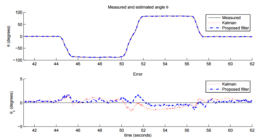
Figure 8. Average results of measurements and estimates of the angle θ (above) and estimation errors (below)


Figure 9. Average results of the measurements and estimates of the angle ψ (above) ) and evaluation errors (below)

5.2. Static and dynamic characteristics

The standard deviations of the angles , and were calculated from the assumption that the angular velocity in the stationary state was <5 ◦ / s and in the mobile state ≥ 5 ◦ / s.

This threshold was chosen so as to be sufficiently high with respect to the noise level of the input data. Each value of the standard deviation was calculated in the time interval in which rotations of the corresponding Euler angle were performed, as shown in Fig. 7, 8 and 9. This was done to prevent errors due to the initial approach or features in the representation of Euler angles, that is, when θ = ± 90 (we are talking about folding frames ). The results are shown in table 1. Each value represents the average of all 8 experiments. The standard deviation values ​​were not calculated for the implementation without a magnetometer, since this implementation is not intended to accurately determine the course and cannot compensate for the accumulation of errors in this parameter.


Table 1. Standard deviations for filters: based on the Kalman method and the proposed method in implementations with and without magnetometer

The results show that the proposed filter achieves higher accuracy than a filter based on the Kalman method. Orientation sensor manufacturers indicate the average deviations of filters based on the Kalman method within <0.5◦ for angles φ and θ and <1◦ for ψ [18]. These values ​​do not correspond to those given in Table 1. Other studies [49] have shown that accuracy can be significantly less than that given by manufacturers and that the level of accuracy indicated by them is achieved only during calibration. The low accuracy levels in measuring the ψ course are caused by the low level of accuracy of the sensor in measuring the Earth's magnetic field. The slope of the Earth’s magnetic field during testing was between 65 ° and 70 ° with respect to the horizon [39]. As a consequence, the components of the magnetic flux vector for determining the course are relatively small. A larger component of the vector, along with the measurement of gravity, serves as an additional criterion for determining the roll θ and pitch φ. Hence pitch standard deviation in pitchand the roll will be less than the rate . The magnetometer, as indicated in [18], has a bandwidth of 10 Hz, which, in comparison with the bandwidth of the accelerometer and gyroscope, which is from 30 to 40 Hz, also implies an increased error in determining the course in a stationary state.

5.3. Effect of filter gain on accuracy

The results of the study of the influence of the gain β on the filter accuracy are displayed in the form of a graph in Fig. 10. The experimental data were processed limited to β values ​​between 0 and 0.5. Each filter implementation has its own optimal value β, which is high enough to compensate for the accumulation of errors and low enough so that unnecessary noise does not fall into large steps of the gradient descent.


Fig. 10. The effect of the gain of the filter β on accuracy

5.4. Influence of measurement frequency on accuracy

In fig. 11 presents the results of a study of the effect of measurement frequency on filter accuracy. The experiments were carried out using the optimal value of the gain β for both implementations (with and without magnetometer). The change in the measurement frequency was simulated by skipping part of the measurements and ranged from 1 Hz to 512 Hz. From fig. 11 you can see that the proposed filter reaches the same level of accuracy at a sampling frequency of 50 Hz, as at a frequency of 512 Hz. Both filter implementations achieve a decrease in the static error (in the stationary state) <2◦ and the dynamic error (in the mobile state of the platform) <7◦ even at a sampling frequency of 10 Hz. This level of accuracy is sufficient for use in human motion capture applications.


Fig. 11. The influence of measurement frequency on filter accuracy for implementations with and without magnetometer

5.5. Gyroscope zero drift

The calibrated gyro data used in the proposed filter does not contain any bias errors. To investigate the ability of the proposed filter to compensate for drift, errors were artificially introduced into the data of all 8 experiments. A constant drift of 0.2◦ / s / s was added to the measurements of the gyroscope along the X axis and a constant bias error of −0.2 ◦ / s / s to the measurements of the gyroscope along the Y axis. The gain ζ was set to 0 during the first 10 seconds during each experiment, until the filter converged with the initial conditions. After that, the value was set to 0.015 as corresponding to the maximum displacement velocity of the gyroscope 1 ° / sec / sec. Fig. 12 shows the average results of 8 experiments, showing the zero bias of the gyroscope according to the filter estimates from the actual position along the axes of the gyroscope X and Y. The accuracy of the filter under these conditions is described in table 1.


Fig. 12 Gyroscope Zero Drift Tracking Filter

6. Discussion

At the beginning of work on the filter, it was assumed that the accelerometer and magnetometer would measure only the gravity and magnetic field of the Earth. In practice, due to accelerations of movement, this leads to an erroneous observed direction of gravity (especially if the overload created by the movement is comparable to or greater than the value of gravity), which gives a potentially incorrect estimate of the height, and distortions of the magnetic field give an incorrect estimate of the course. In many filter implementations, the authors make the assumption that acceleration of motion and magnetic distortions are present only for a short period of time. Therefore, the filter gain β can be chosen low enough so that the deviation caused by erroneous notions of gravitational and magnetic distortions observed locally decreases to an acceptable level over a period. The minimum allowable value of β is limited by the measurement error of the gyroscope.

In many applications, it may be useful to use dynamic increment of β and ζ. This will reduce the influence of the accelerometer or magnetometer on the assessment of the current position during problem periods, for example, when a large overload is detected. Using large filter gain values ​​during initialization can also improve the convergence of the filter under initial conditions. For example, it was found that an increase in β and ζ by 10 allows for 5 seconds from the moment the filter is turned on to compensate for the gyro shift error of 1000 deg / s in each axis.

The filter structure for installing the array of ANN sensors with a magnetometer is similar to that proposed by Bachmann and others [34]. Both filter implementations estimate the gyro measurement error as the gradient of the error surface created by the measurements of the accelerometer and magnetometer. The Bachmann filter computes this using the Gauss-Newton approach, which requires numerical differentiation and matrix inversion. The filter proposed in this report uses the analytical conclusion of Jacobi and operates on a normalized gradient of the error surface. As a result, the filter proposed in this article provides a significant reduction in the computational load and allows the filter to optimally amplify the source, based on the observed characteristics of the system.

The experimental procedure used to evaluate the accuracy of the filter has several limitations. The filter was not rated for simultaneous rotation around more than one axis, and rotation speeds were limited in magnitude and in time. These limitations were necessary so that repeatability and quantification were possible.

7. Conclusions

Essentially a repeat of the text from the introduction.

Appendix A. Filter implementation on C without magnetometer

The following source code is an implementation of an orientation filter without a magnetometer. C. code has been optimized to minimize the required number of arithmetic operations due to RAM. Each scalar filter requires 109 scalar arithmetic operations (18 addition, 20 subtraction, 57 multiplications, 11 divisions and 3 square root). The implementation requires 40 bytes of RAM for global variables and 100 bytes of RAM for local variables during each call filter update functions.

Appendix A. Filter implementation on C with magnetometer

The following source code is an implementation of an orientation filter with a magnetometer and a gyro drift compensation system. C. code has been optimized to minimize the required number of arithmetic operations due to RAM. Each filter update requires 277 scalar arithmetic operations (51 additions, 57 subtractions, 155 multiplications, 14 divisions and 5 square root). The implementation requires 72 bytes of RAM for global variables and 260 bytes of RAM for local variables during each call filter update functions.

List of references

1. Mark Euston, Paul Coote, Robert Mahony, Jonghyuk Kim, and Tarek Hamel. A complementary filter for attitude estimation of a fixed-wing uav with a low-cost imu. In 6th International Conference on Field and Service Robotics, July 2007.
2. Sung Kyung Hong. Fuzzy logic based closed-loop strapdown attitude system for unmanned aerial vehicle (uav). Sensors and Actuators A: Physical, 107(2):109 – 118, 2003.
3. A. Kallapur, I. Petersen, and S. Anavatti. A robust gyroless attitude estimation scheme for a small fixed-wing unmanned aerial vehicle. pages 666 –671, aug. 2009.
4. B. Barshan and H. F. Durrant-Whyte. Inertial navigation systems for mobile robots. 11(3):328–342, June 1995.
5. L. Ojeda and J. Borenstein. Flexnav: fuzzy logic expert rule-based position estimation for mobile robots on rugged terrain. In Proc. IEEE International Conference on Robotics and Automation ICRA ’02, volume 1, pages 317–322, May 11–15, 2002.
6. David H. Titterton and John L. Weston. Strapdown inertial navigation technology. The Institution of Electrical Engineers, 2004.
7. S. Beauregard. Omnidirectional pedestrian navigation for first responders. In Proc. 4th Workshop on Positioning, Navigation and Communication WPNC ’07, pages 33–36, March 22–22, 2007.
8. H. J. Luinge and P. H. Veltink. Inclination measurement of human movement using a 3-d accelerometer with autocalibration. 12(1):112–121, March 2004. [9] Huiyu Zhou and Huosheng Hu. Human motion tracking for rehabilitation–a survey. volume 3, pages 1 – 18, 2008.
9. E. A. Heinz, K. S. Kunze, M. Gruber, D. Bannach, and P. Lukowicz. Using wearable sensors for real-time recognition tasks in games of martial arts — an initial experiment. In Proc. IEEE Symposium on Computational Intelligence and Games, pages 98–102, May 22–24, 2006.
10. J. E. Bortz. A new mathematical formulation for strapdown inertial navigation. (1):61– 66, January 1971.
11. M B Ignagni. Optimal strapdown attitude integration algorithms. In Guidance, Control, and Dynamics, volume 13, pages 363–369, 1990.
12. N. Yazdi, F. Ayazi, and K. Najafi. Micromachined inertial sensors. 86(8):1640–1659, August 1998.
13. R. E. Kalman. A new approach to linear filtering and prediction problems. Journal of Basic Engineering, 82:35–45, 1960.
14. E. Foxlin. Inertial head-tracker sensor fusion by a complementary separate-bias kalman filter. In Proc. Virtual Reality Annual International Symposium the IEEE 1996, pages 185–194,267, March 30–April 3, 1996.
15. H. J. Luinge, P. H. Veltink, and C. T. M. Baten. Estimation of orientation with gyroscopes and accelerometers. In Proc. First Joint [Engineering in Medicine and Biology 21st Annual Conf. and the 1999 Annual Fall Meeting of the Biomedical Engineering Soc.] BMES/EMBS Conference, volume 2, page 844, October 13–16, 1999.
16. J. L. Marins, Xiaoping Yun, E. R. Bachmann, R. B. McGhee, and M. J. Zyda. An extended kalman filter for quaternion-based orientation estimation using marg sensors. In Proc. IEEE/RSJ International Conference on Intelligent Robots and Systems, volume 4, pages 2003–2011, October 29–November 3, 2001.
17. Xsens Technologies B.V. MTi and MTx User Manual and Technical Documentation. Pantheon 6a, 7521 PR Enschede, The Netherlands, May 2009.
18. MicroStrain Inc. 3DM-GX3 -25 Miniature Attutude Heading Reference Sensor. 459 Hurricane Lane, Suite 102, Williston, VT 05495 USA, 1.04 edition, 2009.
19. VectorNav Technologies, LLC. VN -100 User Manual. College Station, TX 77840 USA, preliminary edition, 2009.
20. InterSense, Inc. InertiaCube2+ Manual. 36 Crosby Drive, Suite 150, Bedford, MA 01730, USA, 1.0 edition, 2008.
21. PNI sensor corporation. Spacepoint Fusion. 133 Aviation Blvd, Suite 101, Santa Rosa, CA 95403-1084 USA.
22. Crossbow Technology, Inc. AHRS400 Series Users Manual. 4145 N. First Street, San Jose, CA 95134, rev. c edition, February 2007.
23. A. M. Sabatini. Quaternion-based extended kalman filter for determining orientation by inertial and magnetic sensing. 53(7):1346–1356, July 2006.
24. H. J. Luinge and P. H. Veltink. Measuring orientation of human body segments using miniature gyroscopes and accelerometers. Medical and Biological Engineering and Computing, 43(2):273–282, April 2006.
25. David Jurman, Marko Jankovec, Roman Kamnik, and Marko Topic. Calibration and data fusion solution for the miniature attitude and heading reference system. Sensors and Actuators A: Physical, 138(2):411–420, August 2007.
26. Markus Haid and Jan Breitenbach. Low cost inertial orientation tracking with kalman filter. Applied Mathematics and Computation, 153(4):567 575, June 2004.
27. D. Roetenberg, H. J. Luinge, C. T. M. Baten, and P. H. Veltink. Compensation of magnetic disturbances improves inertial and magnetic sensing of human body segment orientation. 13(3):395–405, September 2005.
28. John L. Crassidis and Landis F. Markley. Unscented filtering for spacecraft attitude estimation. Journal of guidance, control, and dynamics, 26(4):536–542, 2003.
29. D. Gebre-Egziabher, R.C. Hayward, and J.D. Powell. Design of multi-sensor attitude determination systems. Aerospace and Electronic Systems, IEEE Transactions on, 40(2):627 – 649, april 2004.
30. N.H.Q. Phuong, H.-J. Kang, Y.-S. Suh, and Y.-S. Ro. A DCM based orientation estimation algorithm with an inertial measurement unit and a magnetic compass. Journal of Universal Computer Science, 15(4):859–876, 2009.
31. Daniel Choukroun. Novel methods for attitude determination using vector observations. PhD thesis, Israel Institute of Technology, May 2003.
32. R. A. Hyde, L. P. Ketteringham, S. A. Neild, and R. J. S. Jones. Estimation of upperlimb orientation based on accelerometer and gyroscope measurements. 55(2):746–754, February 2008.
33. E. R. Bachmann, I. Duman, U. Y. Usta, R. B. McGhee, X. P. Yun, and M. J. Zyda. Orientation tracking for humans and robots using inertial sensors. In Proc. IEEE International Symposium on Computational Intelligence in Robotics and Automation CIRA
34. ’99, pages 187–194, November 8–9, 1999.
35. R. Mahony, T. Hamel, and J.-M. Pflimlin. Nonlinear complementary filters on the special orthogonal group. Automatic Control, IEEE Transactions on, 53(5):1203 –1218, june 2008.
36. J. B. Kuipers. Quaternions and Rotation Sequences: A Primer with Applications to Orbits, Aerospace and Virtual Reality. Princeton University Press, 1999.
37. John J. Craig. Introduction to Robotics Mechanics and Control. Pearson Education International, 2005.
38. David R. Pratt Robert B. McGhee Joseph M. Cooke, Michael J. Zyda. Npsnet: Flight simulation dynamic modelling using quaternions. Presence, 1:404–420, 1994.
39. John Arthur Jacobs. The earth’s core, volume 37 of International geophysics series. Academic Press, 2 edition, 1987.
40. E. R. Bachmann, Xiaoping Yun, and C. W. Peterson. An investigation of the effects of magnetic variations on inertial/magnetic orientation sensors. In Proc. IEEE International Conference on Robotics and Automation ICRA ’04, volume 2, pages 1115–1122, April 2004.
41. C.T.M. Baten F.C.T. van der Helm W.H.K. de Vries, H.E.J. Veeger. Magnetic distortion in motion labs, implications for validating inertial magnetic sensors. Gait & Posture, 29(4):535–541, 2009.
42. Speake & Co Limited. Autocalibration algorithms for FGM type sensors. Application note.
43. Michael J. Caruso. Applications of Magnetoresistive Sensors in Navigation Systems. Honeywell Inc., Solid State Electronics Center, Honeywell Inc. 12001 State Highway 55, Plymouth, MN 55441.
44. J. F. Vasconcelos, G. Elkaim, C. Silvestre, P. Oliveira, and B. Cardeira. A geometric approach to strapdown magnetometer calibration in sensor frame. In Navigation, Guidance and Control of Underwater Vehicles, volume 2, 2008.
45. Demoz Gebre-Egziabher, Gabriel H. Elkaim, J. David Powell, and Bradford W. Parkinson. Calibration of strapdown magnetometers in magnetic field domain. Journal of Aerospace Engineering, 19(2):87–102, 2006.
46. Vicon Motion Systems Limited. Vicon MX Hardware. 5419 McConnell Avenue, Los Angeles, CA 90066, USA, 1.6 edition, 2004.
47. Vicon Motion Systems Limited. Vicon Nexus Product Guide — Foundation Notes. 5419 McConnell Avenue, Los Angeles, CA 90066, USA, 1.2 edition, November 2007.
48. Itzhack Y Bar-Itzhack. New method for extracting the quaternion from a rotation matrix. AIAA Journal of Guidance, Control and Dynamics, 23(6):10851087, Nov.Dec 2000. (Engineering Note).
49. MA Brodie, A. Walmsley, and W. Page. The static accuracy and calibration of inertial measurement units for 3D orientation. Computer Methods in Biomechanics and Biomedical Engineering, 11 (6): 641–648, December 2008.