Hybrid implementation of the MST algorithm using CPU and GPU

Introduction

Solving the problem of searching for minimum spanning trees (MST - minimum spanning tree) is a common task in various fields of research: recognition of various objects, computer vision, analysis and construction of networks (for example, telephone, electrical, computer, road, etc.), chemistry and biology and many others. There are at least three well-known algorithms that solve this problem: Boruvki, Kruskal and Prima. Processing large graphs (occupying several GB) is a rather time-consuming task for the central processor (CPU) and is in demand at this time. Graphics accelerators (GPUs), capable of showing much greater performance than CPUs, are becoming more widespread. But the MST task, like many graph processing tasks, does not fit well with the GPU architecture. This article will discuss the implementation of this algorithm on the GPU. It will also be shown how the CPU can be used to build a hybrid implementation of this algorithm on the shared memory of one node (consisting of a GPU and several CPUs).

Description of the graph presentation format

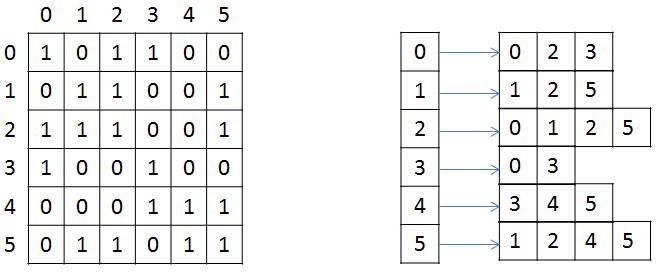
We briefly consider the storage structure of an undirected weighted graph, since in the future it will be mentioned and transformed. The graph is set in compressed CSR (Compressed Sparse Row) [1]format. This format is widely used for storing sparse matrices and graphs. For a graph with N vertices and M edges, three arrays are needed: X, A and W. Array X is of size N + 1, the other two are 2 * M, since in a non-oriented graph for any pair of vertices it is necessary to store the forward and backward arcs. Array X stores the beginning and end of the list of neighbors that are stored in array A, that is, the entire list of neighbors of the vertex J is in array A from index X [J] to X [J + 1], not including it. The similar indices store the weights of each edge from the vertex J. For illustration, the figure below shows the graph of 6 vertices written using the adjacency matrix, and the CSR format on the right (for simplicity, the weight of each edge is not indicated).

Tested Graphs

I will immediately describe on which graphs the testing took place, since a description of the transformation algorithms and the MST algorithm will require knowledge of the structure of the graphs in question. Two types of synthetic graphs are used to evaluate implementation performance: RMAT graphs and SSCA2 graphs. R-MAT-graphs well model real graphs from social networks, the Internet [2] . In this case, we consider RMAT graphs with an average degree of connectedness of the vertex 32, and the number of vertices is a power of two. Such an RMAT graph has one large connected component and a number of small connected components or hanging vertices. SSCA2-graph is a large set of independent components connected by edges with each other [3]. The SSCA2 graph is generated so that the average degree of connectivity of the vertex is close to 32, and its number of vertices is also a power of two. Thus, two completely different graphs are considered.

Input Conversion

Since the testing of the algorithm will be carried out on the RMAT and SSCA2 graphs, which are obtained using the generator, some transformations are necessary to improve the performance of the algorithm. All conversions will not be included in the performance calculation.

1. Local sorting of the list of vertices
   For each vertex, we sort its list of neighbors by weight, in ascending order. This will partially simplify the choice of the minimum edge at each iteration of the algorithm. Since this sorting is local, it does not provide a complete solution to the problem.
   
2. Renumbering all vertices of the graph
   We number the vertices of the graph so that the most connected vertices have the closest numbers. As a result of this operation, in each connected component, the difference between the maximum and minimum vertex number will be the smallest, which will allow the best use of the small graphics process cache. It is worth noting that for RMAT graphs, this renumbering does not have a significant effect, since there is a very large component in this graph that does not fit into the cache even after applying this optimization. For SSCA2 graphs, the effect of this transformation is more noticeable, since in this graph there are a large number of small components.
   
3. Mapping graph weights to integers
   In this problem, we do not need to perform any operations on the graph weights. We need to be able to compare the weights of two ribs. For these purposes, you can use integers instead of double precision numbers, since the processing speed of single precision numbers on the GPU is much higher than double. This transformation can be performed for graphs whose number of unique edges does not exceed 2 ^ 32 (the maximum number of different numbers that fit in an unsigned int). If the average degree of connectivity of each vertex is 32 m, then the largest graph that can be processed using this transformation will have 2 ^ 28 vertices and will occupy 64 GB in memory. To date, the largest amount of memory in accelerators NVidia Tesla k40 [4] / NVidia Titan X[5] and AMD FirePro w9100 [6] are 12GB and 16GB respectively. Therefore, on a single GPU using this conversion, you can process quite large graphs.
   
4. Vertex Compression
   This transformation is applicable only to SSCA2 graphs due to their structure. In this problem, the decisive role is played by the memory performance of all levels: from global memory to the first level cache. To reduce the traffic between the global memory and the L2 cache, you can store vertex information in a compressed form. Initially, information about vertices is presented in the form of two arrays: array X, which stores the beginning and end of the list of neighbors in array A (an example for only one vertex):
   
   Vertex J has 10 neighbor vertices, and if the number of each neighbor is stored using the unsigned int type, then 10 * sizeof (unsigned int) bytes are required to store the list of neighbors of the J vertex, and 2 * M * sizeof (unsigned for the entire graph) int) byte. We assume that sizeof (unsigned int) = 4 bytes, sizeof (unsigned short) = 2 bytes, sizeof (unsigned char) = 1 byte. Then for this vertex, 40 bytes are needed to store the list of neighbors.
   It is not difficult to notice that the difference between the maximum and minimum number of the vertex in this list is 8, and only 4 bits are needed to store this number. Based on those considerations that the difference between the maximum and minimum number of a vertex can be less than unsigned int, we can represent the number of each vertex as follows:
   base_J + 256 * k + short_endV,
   where base_J is, for example, the minimum vertex number from the entire list of neighbors. In this example, it will be 1. This variable will be of type unsigned int and there will be as many such variables as there are vertices in the graph; Next, we calculate the difference between the vertex number and the selected base. Since we chose the smallest peak as the base, this difference will always be positive. For SSCA2, this difference will be placed in unsigned short. short_endV is the remainder of dividing by 256. To store this variable, we will use the unsigned char type; and k is the integer partfrom dividing by 256. For k, select 2 bits (that is, k lies in the range from 0 to 3). The selected representation is sufficient for the graph in question. In the bit representation, it looks like this:
   
   Thus, to store the list of vertices, (1 + 0.25) * 10 + 4 = 16.5 bytes are required for this example, instead of 40 bytes, and for the entire graph: (2 * M + 4 * N + 2 * M / 4) instead of 2 * M * 4. If N = 2 * M / 32, then the total volume will decrease in
   (8 * M) / (2 * M + 8 * M / 32 + 2 * M / 4) = 2.9 times
   

General description of the algorithm

To implement the MST algorithm, the Boruwka algorithm was chosen. The basic description of the Boruwka algorithm and an illustration of its iterations are well presented here [7] .
According to the algorithm, all vertices are initially included in the minimal tree. Next, you must follow these steps:

1. Find the minimum edges between all the trees for their subsequent union. If no edges are selected at this step, then the answer to the problem is received
2. Merge matching trees. This step is divided into two stages: deleting cycles, since two trees can indicate each other as a candidate for merging, and the merging step when the number of the tree that includes the combined subtrees is selected. For definiteness, we will choose the minimum number. If only one tree remains during the merge, then the answer to the problem is received.
3. Renumber the resulting trees to go to the first step (so that all trees have numbers from 0 to k)

Algorithm Stages

In general, the implemented algorithm is as follows:

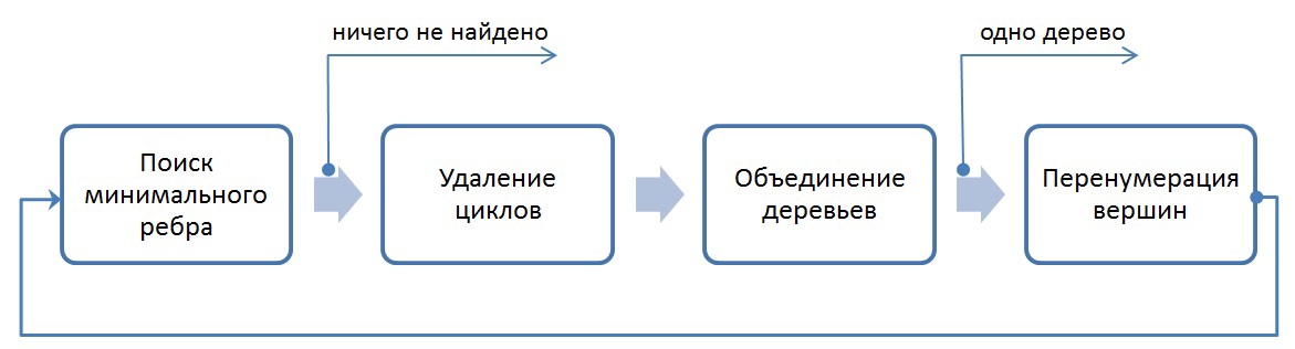
The exit from the entire algorithm occurs in two cases: if all vertices after N iterations are combined into one tree, or if it is impossible to find the minimum edge from each tree (in this case, the minimum spanning trees are found).

1. Search for the minimum edge.

First, each vertex of the graph is placed in a separate tree. Next, an iterative process of combining trees occurs, consisting of the four procedures discussed above. The procedure for finding the minimum edge allows you to select exactly those edges that will be included in the minimum spanning tree. As described above, at the input of this procedure, the converted graph is stored in CSR format. Since the edges were partially sorted by weight for the list of neighbors, the choice of the minimum vertex is reduced to viewing the list of neighbors and selecting the first vertex that belongs to another tree. If we assume that there are no loops in the graph, then at the first step of the algorithm, choosing the minimum vertex reduces to choosing the first vertex from the list of neighbors for each vertex under consideration, because the list of neighboring vertices (which make up the edges of the graph together with the vertex under consideration) is sorted by increasing the weight of the edges, and each vertex is included in a separate tree. At any other step, you need to look through the list of all neighboring vertices in order and select the vertex that belongs to another tree.

Why is it impossible to select the second vertex from the list of neighboring vertices and put this edge minimal? After the procedure of combining trees (which will be considered later), a situation may arise that some vertices from the list of neighboring ones may appear in the same tree as the one under consideration, thereby this edge will be a loop for this tree, and by the condition of the algorithm, it is necessary to choose the minimum edge to other trees.

Union Find is a good fit for implementing vertex processing and performing the search, merge and merge lists. [8]. Unfortunately, not all structures are optimally processed on the GPU. The most profitable in this task (as in most others) is to use continuous arrays in the GPU memory, instead of linked lists. Below we will consider similar algorithms for finding the minimum edge, combining segments, deleting cycles in the graph.

Consider the algorithm for finding the minimum edge. It can be represented in two steps:

• selection of the minimum edge outgoing from each vertex (which is included in some segment) of the graph in question;
• selection of edges of minimum weight for each tree.

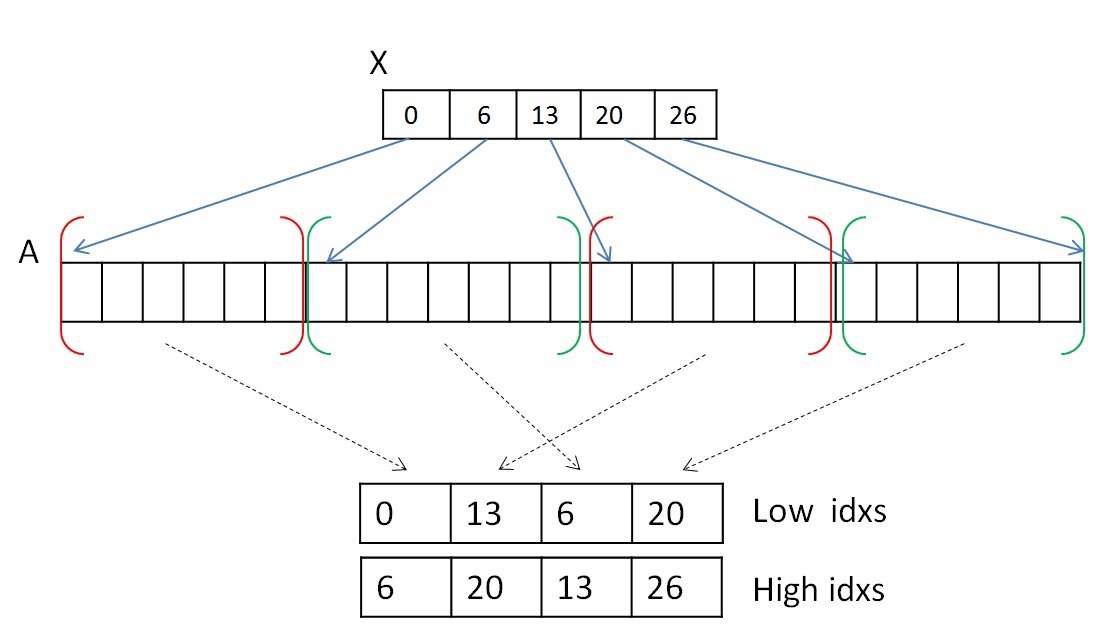
In order not to move the vertex information recorded in CSR format, we will use two auxiliary arrays that will store the index of the beginning and end of array A of the neighbor list. Two given arrays will indicate segments of vertex lists belonging to one tree. For example, in the first step, the array of beginnings or lower values ​​will have the values ​​0..N of the array X, and the array of ends or the upper values ​​will have the values ​​1..N + 1 of the array X. And then, after the procedure of combining trees (which will be considered later ), these segments are mixed, but the array of neighbors A will not be changed in memory.

Both steps can be performed in parallel. To complete the first step, you need to look at the list of neighbors of each vertex (or each segment) and select the first edge belonging to another tree. You can select one warp (consisting of 32 threads) to view a list of neighbors of each vertex. It is worth remembering that several segments of the array of neighboring peaks A can lie not in a row and belong to one tree (the segments belonging to tree 0 are highlighted in red and the tree 1 is highlighted in green):

Due to the fact that each segment of the list of neighbors is sorted, it is not necessary to view all the vertices. Since one warp consists of 32 threads, viewing will be done in portions of 32 vertices. After 32 vertices are viewed, you need to combine the result and if nothing is found, then view the next 32 vertices. To combine the result, you can use the scan algorithm [9] . It is possible to implement this algorithm inside one warp using shared memory or using new shfl instructions [10](available from the Kepler architecture), which allow the exchange of data between the threads of one warp for one instruction. As a result of the experiments, it turned out that shfl-instructions can speed up the work of the entire algorithm by about two times. Thus, this operation can be performed using shfl instructions, for example, like this:

	unsigned idx = blockIdx.x * blockDim.x + threadIdx.x; // глобальный индекс нити
	unsigned lidx = idx % 32;  
#pragma unroll
	for (int offset = 1; offset <= 16; offset *= 2)
	{
		tmpv = __shfl_up(val, (unsigned)offset);
		if(lidx >= offset)
			val += tmpv;
	}
	tmpv = __shfl(val, 31); // рассылка всем нитям последнего значения. Если получено значение 1, то какая-то нить нашла 
                            // минимальное ребро, иначе необходимо продолжить поиск.

As a result of this step, the following information will be recorded for each segment: the number of the vertex in array A that is included in the edge of minimum weight and the weight of the edge itself. If nothing is found, then, for example, the number N + 2 can be written in the vertex number.

The second step is necessary to reduce the selected information, namely, the choice of edges with a minimum weight for each of the trees. This step is done because segments belonging to the same tree are scanned in parallel and independently, and a minimum weight edge is selected for each segment. In this step, one warp can reduce information for each tree (for several segments), and shfl instructions can also be used for reduction. After completing this step, it will be known with which tree each of the trees is connected by a minimal edge (if it exists). To record this information, we introduce two more auxiliary arrays, in one of which we will store the numbers of trees up to which there is a minimum edge, in the second - the number of the vertex in the original graph, which is the root of the vertices entering the tree.

It is worth noting that to work with indexes, two more arrays are needed, which help to convert the original indexes into new indexes and get the original index using the new index. These so-called index conversion tables are updated with each iteration of the algorithm. The table for obtaining a new index by the initial index has the size N - the number of vertices in the graph, and the table for obtaining the initial index is reduced in a new way with each iteration and has a size equal to the number of trees in any chosen iteration of the algorithm (at the first iteration of the algorithm, this table also has size N).

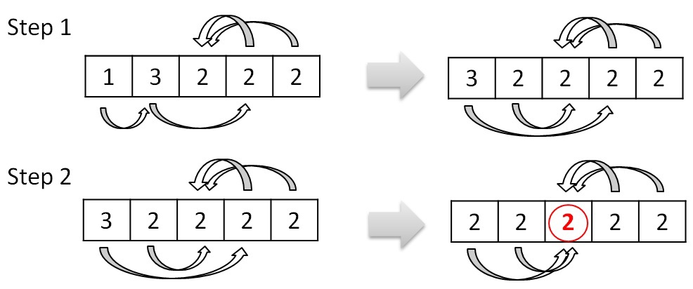
2. Delete cycles.

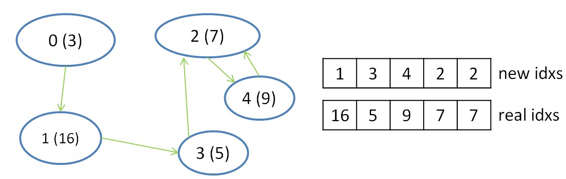
This procedure is necessary to remove loops between two trees. This situation occurs when the tree N1 has a minimal edge to the tree N2, and the tree N2 has the minimum edge to the tree N1. In the picture above, there is a cycle only between two trees with numbers 2 and 4. Since there are fewer trees at each iteration, we will choose the minimum number of two trees that make up the cycle. In this case, 2 will point to 2, and 4 will continue to point to 2. Using these checks, you can determine such a cycle and eliminate it in favor of the minimum number:

    unsigned i = blockIdx.x * blockDim.x + threadIdx.x;
    unsigned local_f = сF[i]; 
    if (сF[local_f] == i)
    {
         if (i < local_f)
         {
                F[i] = i;
                . . . . . . .  
          }
    }

This procedure can be performed in parallel, since each vertex can be processed independently and records in a new array of vertices without cycles do not intersect.

3. The union of trees.

This procedure combines the trees into larger ones. The procedure for deleting loops between two trees is essentially a preprocessing before this procedure. It avoids looping when merging trees. Combining trees is the process of choosing a new root by changing links. If, for example, tree 0 points to tree 1, and tree 1 in turn points to tree 3, then you can change the link of tree 0 from tree 1 to tree 3. This link change is worthwhile if changing the link does not result in a loop between the two trees . Considering the example above, after the procedures for deleting cycles and merging trees, only one tree with number 2 remains. The process of combining can be represented like this:

The structure of the graph and the principle of its processing are such that there will be no situation where the procedure will loop and it can also be performed in parallel.

4. Renumbering peaks (trees).

After the union procedure is completed, it is necessary to renumber the resulting trees so that their numbers go in a row from 0 to P. By construction, the new numbers must receive array elements that satisfy the condition F [i] == i (for the example considered above, only the element satisfies this condition with index 2). Thus, using atomic operations, you can mark the entire array with new values ​​from 1 ... (P + 1). Next, complete the tables for obtaining a new index by the initial and the initial index in a new way:

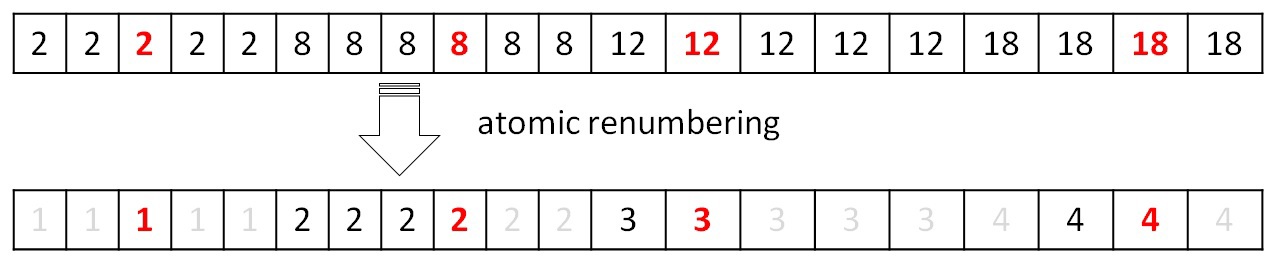
Working with these tables is described in the procedure for finding the minimum edge. The next iteration cannot be performed correctly without updating the table data. All described operations are performed in parallel and on the GPU.

To summarize. All 4 procedures are performed in parallel and on a graphics accelerator. Work is being done with one-dimensional arrays. The only difficulty is that all of these procedures have indirect indexing. And in order to reduce cache misses from such work with arrays, various permutations of the graph described at the very beginning were used. But, unfortunately, not every graph manages to reduce losses from indirect indexing. As will be shown later, with this approach, RMAT graphs achieve not very high performance. Finding the minimum edge takes up to 80% of the running time of the entire algorithm, while the rest accounts for the remaining 20%. This is due to the fact that in the procedures of combining, deleting loops, and renumbering vertices, work is carried out with arrays whose length is constantly decreasing (from iteration to iteration). For the considered graphs, it is necessary to do about 7-8 iterations. This means that the number of vertices to be processed already at the first step becomes much less than N / 2. While in the main procedure for finding the minimum edge, work is done with arrays of vertices A and an array of weights W (although certain elements are selected).
In addition to storing the graph, several more arrays of length N were used:

• an array of lower values ​​and an array of upper values. Used to work with segments of array A;
• array-table to get the original index on a new one;
• array-table to get a new index on the original;
• an array for vertex numbers and an array for the weights corresponding to them, which are used in the second step of the minimum edge search procedure;
• auxiliary array that allows you to determine in the first step of the procedure for finding the minimum edge to which tree this or that segment belongs.

Hybrid implementation of the minimal edge search procedure.

The algorithm described above ultimately does not perform poorly on a single GPU. The solution to this problem is organized in such a way that you can try to parallelize this procedure also on the CPU. Of course, this can only be done on shared memory, and for this I used the OpenMP standard and transfer data between the CPU and GPU via the PCIe bus. If you imagine the execution of procedures at one iteration on the time line, then the picture when using one GPU will be something like this:

Initially, all graph data is stored both on the CPU and on the GPU. In order for the CPU to be able to read, it is necessary to transmit information about segments moved during the merging of trees. Also, in order for the GPU to continue the iteration of the algorithm, it is necessary to return the calculated data. It would be logical to use asynchronous copying between the host and the accelerator:

The algorithm on the CPU repeats the algorithm used on the GPU, only OpenMP is used to parallelize the loop [11]. As expected, the CPU does not count as fast as the GPU, and the overhead of copying also interferes. In order for the CPU to manage to calculate its part, the data for the calculation should be divided in a ratio of 1: 5, that is, no more than 20% -25% should be transferred to the CPU, and the rest should be calculated on the GPU. The rest of the procedures are not advantageous to consider both here and there, since they take very little time, and the overhead and slow CPU speed only increase the algorithm time. The copy speed between the CPU and GPU is also very important. The tested platform supported PCIe 3.0, which allowed reaching 12GB / s.

To date, the amount of RAM on the GPU and CPU is significantly different in favor of the latter. On the test platform, 6 GB GDDR5 was installed, while on the CPU there were as many as 48 GB. The memory limits on the GPU do not allow the calculation of large graphs. And here the CPU and Unified Memory technology can help us [12], which allows you to access the GPU in the CPU memory. Since information about the graph is necessary only in the procedure for finding the minimum edge, for large graphs, you can do the following: first place all the auxiliary arrays in the GPU memory, and then place part of the graph arrays (array of neighbors A, array X and array of weights W) in memory GPU, but what did not fit - in the memory of the CPU. Further, during the calculation, it is possible to divide the data so that the part that does not fit on the GPU is processed on the CPU, and the GPU minimally uses access to the CPU memory (since access to the CPU memory from the graphics accelerator is through the PCIe bus at a speed of no more 15 GB / s). It is known in advance in what proportion the data was divided, so in order to determine which memory you need to access - in the GPU or CPU - just enter a constant, showing at which point the arrays are separated and with a single check in the algorithm on the GPU, you can determine where to call. The location in memory of these arrays can be represented approximately like this:

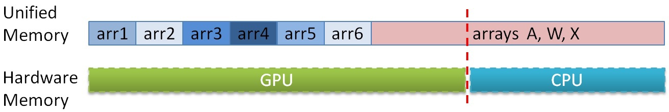
Thus, it is possible to process graphs that do not initially fit on the GPU even when using the described compression algorithms, but at a lower speed, since PCIe throughput is very limited.

Test results

Testing was performed on the NVidia GTX Titan GPU, which has 14 SMX with 192 cuda cores (2688 in total) and a 6 cores (12th) Intel Xeon E5 v1660 processor with a frequency of 3.7 GHz. The graphs on which the tests were performed are described above. I will give only some characteristics:

Scale (2 ^ N)	Number of vertices	Number of Ribs (2 * M)		Graph Size, GB
		RMAT	SSCA2
16	65,536	2 097 152	~ 2 100 000	~ 0.023
21	2 097 152	67 108 864	~ 67,200,000	~ 0.760
24	16 777 216	536 870 912	~ 537 million	~ 6.3
25	33 554 432	1,073,741,824	~ 1,075,000,000	~ 12.5
26	67 108 864	2 147 483 648	~ 2 150 000 000	~ 25.2
27	134 217 728	4,294,967,296	~ 4,300,000,000	~ 51.2

It can be seen that the graph of scale 16 is quite small (about 25 MB) and even without transformations it easily fits into the cache of one modern Intel Xeon processor. And since the graph weights occupy 2/3 of the total, it is actually necessary to process about 8 MB, which is only about 5 times the L2 GPU cache. However, large graphs require a sufficient amount of memory, and even a graph of scale 24 can no longer fit into the memory of the tested GPU without compression. Based on the graph representation, 26 is the last scale, in which the number of edges is placed in unsigned int, which is some limitation of the algorithm for further scaling. This limitation is easily bypassed by expanding the data type. It seems to me that this is not so relevant so far, since processing single precision (unsigned int) is many times faster, than double (unsigned long long) and the amount of memory is still small enough. Performance will be measured in the number of edges processed per second (traversed edges per second - TEPS).

Compilation was carried out using the NVidia CUDA Toolkit 7.0 with options -O3 -arch = sm_35, Intel Composer 2015 with options -O3. The maximum performance of the implemented algorithm can be seen in the graph below:

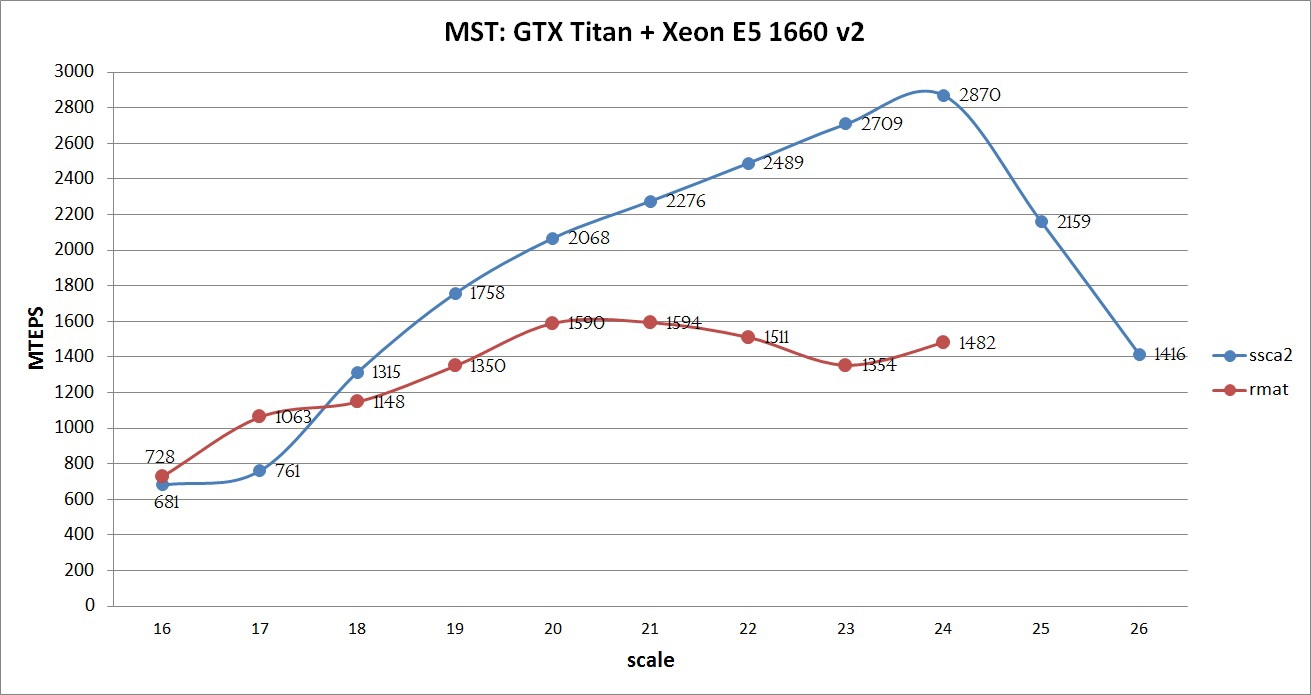
The graph shows that, using all the SSCA2 optimizations, the graphs show good performance: the larger the graph, the better the performance. This growth is maintained until all the data is stored in the GPU memory. At 25 and 26 scales, the Unified Memory mechanism was used, which allowed to obtain a result, albeit at a lower speed (but as will be shown below, faster than only on the CPU). If the calculation were performed on a Tesla k40 with 12GB of memory and disabled ECC and Intel Xeon E5 V2 / V3 processor, then it would be possible to achieve about 3000 MTEPS on a SSCA2 graph of scale 25, and also try to process not only a graph of the 26th scale, but also 27. Such an experiment was not conducted for the RMAT graph, due to its complex structure and poor adaptation of the algorithm.

Comparison of the performance of various algorithms

This problem was solved in the framework of the competition of the GraphHPC 2015 conference. I would like to give a comparison with the program written by Alexander Daryin, who, according to the authors, took first place in this competition.
Since the general table contains the results on the test platform provided by the authors, it would not be out of place to bring graphics on the CPU and GPU on the described platform (GTX Titan + Xeon E5 v2). Below are the results for two graphs:



It can be seen from the graphs that the algorithm described in this article is more optimized for SSCA2 graphs, while the algorithm implemented by Alexander Daryin is well optimized for RMAT graphs. In this case, it is impossible to say unequivocally which of the implementations is the best, because each has its own advantages and disadvantages. Also, the criterion by which algorithms should be evaluated is not clear. If we talk about processing large graphs, then the fact that the algorithm can process graphs of 24-26 scale is a big plus and advantage. If we talk about the average processing speed of graphs of any size, it is not clear which average value to consider. Only one thing is clear - one algorithm handles SSCA2 graphs well, the second - RMAT. If you combine these two implementations, then the average performance will be about 3200 MTEPS for 23 scale. The presentation of the description of some optimizations of the algorithm of Alexander Darin can be viewedhere .

From foreign articles, the following can be distinguished.
1) [13] From this article, some ideas were used in the implementation of the described algorithm. It is impossible to directly compare the results obtained by the authors, since testing was carried out on the old NVidia Tesla S1070. The performance achieved by the authors on the GPU ranges from 18-36 MTEPS. Published in 2009 and 2013.
2) [14] implementation of the Prim algorithm on the GPU.
3) [15] implementation of k NN-Boruvka on the GPU.
There are also some parallel implementations on the CPU. But I could not find high performance in foreign articles. Maybe one of the readers will be able to tell if I missed something. It is also worth noting that in Russia there are practically no publications on this topic (with the exception of Vadim Zaitsev ), which is very sad, it seems to me.

About the competition and instead of the conclusion

I would like to write my opinion about the past and mentioned competition for the best implementation of MST. These notes are not required to be read and express my personal opinion. It is possible that someone thinks very differently.

The basis for solving this problem for all participants was laid, in fact, the same Boruvka algorithm. It turns out that the task has been simplified a bit, since other algorithms (Kruskal and Prima) have great computational complexity and are slow or poorly mapped onto parallel architectures, including the GPU. It logically follows from the name of the conference that it is necessary to write an algorithm that handles large graphs well, such graphs that, say, occupy 1 GB or more in memory (such graphs have scales of 22 or more). Unfortunately, for some reason, the authors did not take this fact into account and the whole competition came down to writing an algorithm that works well in the cache, as the test platform contained 2 CPUs with a total cache of 50 MB (graphs weighing up to 17 scale <= 50 MB). Only one of the participants showed an acceptable result - Vadim Zaitsev, received a fairly high average value on 2x CPU on graph 22 of the scale. But as it turned out during the conference, this participant has been engaged in the MST task for quite some time. It is likely that the processing speed of large graphs of other implemented algorithms will not be large and will differ greatly from those numbers (for the worse) published on the contest website. It is also worth paying attention to the fact that the graph structures are very different, and why it is suddenly necessary to consider the average value of performance precisely as the arithmetic average is also not entirely clear. The size of the processed graph was also not taken into account. Another unpleasant “feature” of the provided system (which included 2x Intel Xeon E5-2690 and NVidia Tesla K20x) is not working PCIe 3.0 (although it is supported on the GPU and is present on the server board). As a result

It should be noted that solving such problems on the GPU is not easy, since graph processing is difficult to parallelize on the GPU due to architectural features. And it is quite possible that these competitions should contribute to the development of specialists in the field of writing algorithms using non-structural grids for graphic processors. But judging by the results of this year, as well as the previous one, the use of the GPU in such tasks, unfortunately, is very limited.

References:

[1] en.wikipedia.org/wiki/Sparse_matrix
[2] www.dislab.org/GraphHPC-2014/rmat-siam04.pdf
[3] www.dislab.org/GraphHPC-2015/SSCA2-TechReport.pdf
[4 ] www.nvidia.ru/object/tesla-supercomputer-workstations-ru.html
[5] www.nvidia.ru/object/geforce-gtx-titan-x-ru.html#pdpContent=2
[6] www.amd .com / ru-ru / products / graphics / workstation / firepro-3d / 9100
[7] en.wikipedia.org/wiki/Bor%C5%AFvka 's_algorithm
[8] www.cs.princeton.edu/~rs/ AlgsDS07 / 01UnionFind.pdf
[9] habrahabr.ru/company/epam_systems/blog/247805
[10]on-demand.gputechconf.com/gtc/2013/presentations/S3174-Kepler-Shuffle-Tips-Tricks.pdf
[11] openmp.org/wp
[12] devblogs.nvidia.com/parallelforall/unified-memory-in- cuda-6
[13] stanford.edu/~vibhavv/papers/old/Vibhav09Fast.pdf
[14] ieeexplore.ieee.org/xpl/login.jsp?tp=&arnumber=5678261&url=http%3A%2F%2Fieeexplore.ieee .org% 2Fxpls% 2Fabs_all.jsp% 3Farnumber% 3D5678261
[15] link.springer.com/chapter/10.1007%2F978-3-642-31125-3_6