Identify fraud using Enron dataset. Part 2, the search for the optimal model

I present to you the second part of the article on the search for suspected fraud on the basis of data from Enron Dataset. If you have not read the first part, you can read it here .

Now we will talk about the process of building, optimizing and choosing a model that will give the answer: is it worth to suspect a person of fraud?

Earlier, we analyzed one of the open datasets that gives information about suspects in the Enron case and fraud. The offset in the original data was also corrected, gaps (NaN) were filled, after which the data were normalized and the signs were selected.

The result was familiar to many:

• X_train and y_train - sample used for training (111 entries);
• X_test and y_test is the sample on which the predictions of our models will be checked (28 records).

Speaking of models ... In order to correctly predict whether a person should be suspected, based on some signs that characterize his activity, we will use the classification. The main types of models used to solve problems in this segment can be taken from Sklearn:

• Naive Bayes (naive Bayes classifier);
• SVM (support vector machine);
• K-nearest neighbors (nearest neighbors search method);
• Random Forest (random forest);
• Neural Network (neural networks).

There is also a picture that illustrates their applicability quite well:

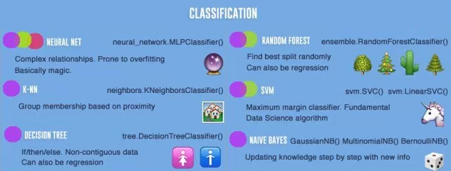
Among them there is a familiar Decision Tree (decision tree), but perhaps there is no point in using this method together with Random Forest, which is an ensemble of decision trees , in one task . Therefore, we replace it with the Logistic Regression (logistic regression), which is able to act as a classifier and produce one of the expected options (0 or 1).

Start

We initialize all mentioned classifiers with default values:

from sklearn.naive_bayes import GaussianNB
from sklearn.linear_model import LogisticRegression
from sklearn.neighbors import KNeighborsClassifier
from sklearn.svm import SVC
from sklearn.neural_network import MLPClassifier
from sklearn.ensemble import RandomForestClassifier
random_state = 42
gnb = GaussianNB()
svc = SVC()
knn = KNeighborsClassifier()
log = LogisticRegression(random_state=random_state)
rfc = RandomForestClassifier(random_state=random_state)
mlp = MLPClassifier(random_state=random_state)

We will also group them in order to make it easier to work with them as with an aggregate, rather than writing code for each one individually. For example, we can train them all at once:

classifiers = [gnb, svc, knn, log, rfc, mlp]
for clf in classifiers:
    clf.fit(X_train, y_train)

After the models have been trained, it's time to first check their prediction quality. Additionally, we visualize our results using Seaborn:

from sklearn.metrics import accuracy_score
defcalculate_accuracy(X, y):
    result = pd.DataFrame(columns=['classifier', 'accuracy'])
    for clf in classifiers:
        predicted = clf.predict(X_test)
        accuracy = round(100.0 * accuracy_score(y_test, predicted), 2)
        classifier = clf.__class__.__name__
        classifier = classifier.replace('Classifier', '')
        result = result.append({'classifier': classifier, 'accuracy': accuracy}, ignore_index=True)
        print('Accuracy is {accuracy}% for {classifier_name}'.format(accuracy=accuracy, classifier_name=classifier))
    result = result.sort_values(['classifier'], ascending=True)
    plt.subplots(figsize=(10, 7))
    sns.barplot(x="classifier", y='accuracy', palette=cmap, data=result)

Let's look at the general idea of ​​the accuracy of the classifiers:

calculate_accuracy(X_train, y_train)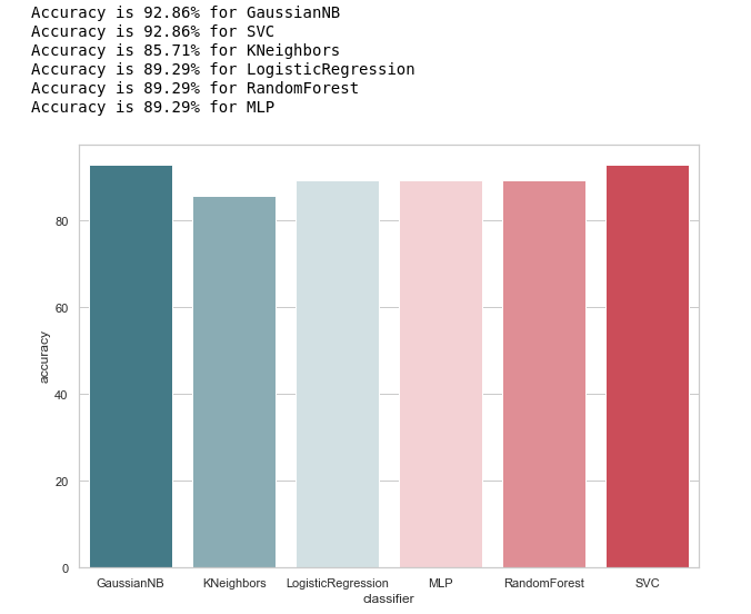 

At first glance, it looks quite good, the accuracy of predictions on the test sample varies around 90%. It seems that the task is done brilliantly!

defQuaziAlgo(features):
    return0

But still, before flattering ourselves, let's build an error confusion matrix for the prediction results:

from sklearn.metrics import confusion_matrix
defmake_confussion_matrices(X, y):
    matrices = {}
    result = pd.DataFrame(columns=['classifier', 'recall'])
    for clf in classifiers:
        classifier = clf.__class__.__name__
        classifier = classifier.replace('Classifier', '')
        predicted = clf.predict(X_test)
        print(f'{predicted}-{classifier}')
        matrix = confusion_matrix(y_test,predicted,labels=[1,0])
        matrices[classifier] = matrix.T
    return matrices

We calculate the error matrix for each classifier and at the same time we will see what they predicted:

matrices = make_confussion_matrices(X_train,y_train)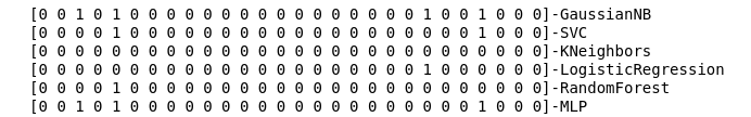

Even a textual representation of the result of the work of the classifiers is enough to understand that something obviously went wrong.

The method of the nearest neighbors did not reveal a single suspect in the test sample at all. There are two questions:

1. What is the reason for such behavior of the KNeighbors classifier?
2. Why did we build error matrices if we do not use them, but simply look at the results of the prediction?

Look deeper

Let's start with the second question. Let's try to visualize our error matrices, and present the data in graphical format to understand where the classification error occurs:

import itertools
from collections import Iterable
def draw_confussion_matrices(row,col,matrices,figsize = (16,12)):
    fig, (axes) = plt.subplots(row,col, sharex='col', sharey='row',figsize=figsize )
    ifany(isinstance(i, Iterable) for i in axes):
        axes =  list(itertools.chain.from_iterable(axes))
    idx = 0forname,matrix in matrices.items():
        df_cm = pd.DataFrame(
            matrix, index=['True','False'], columns=['True','False'], 
        )
        ax = axes[idx]
        fig.subplots_adjust(wspace=0.1)
        sns.heatmap(df_cm, annot=True,cmap=cmap,cbar=False ,fmt="d",ax=ax,linewidths=1) 
        ax.set_title(name)
        idx += 1

Let's display them in 2 rows and 3 columns:

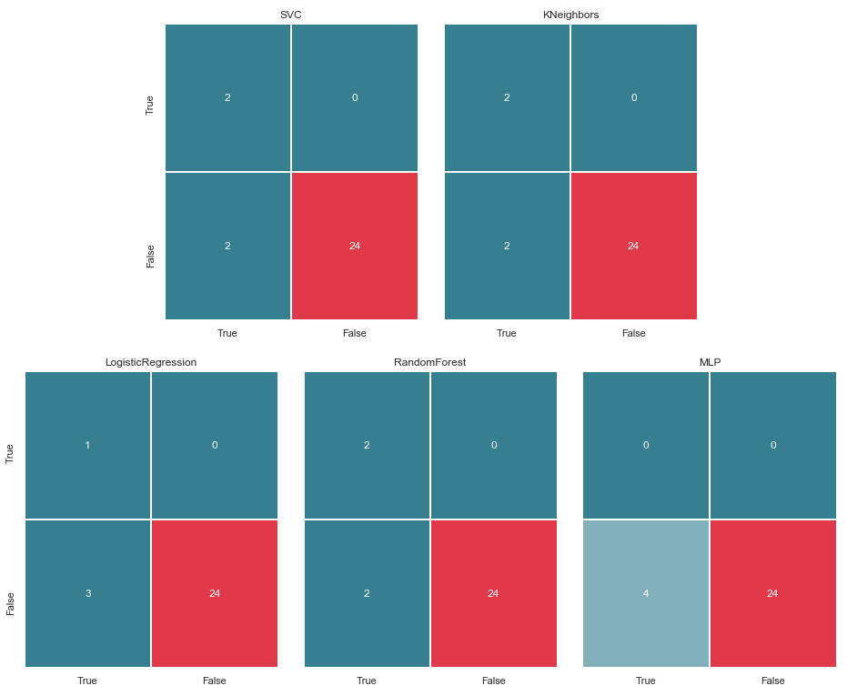
draw_confussion_matrices(2,3,matrices)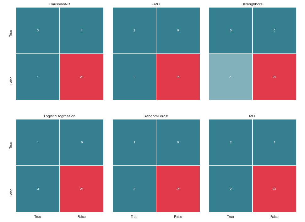

Before continuing, it is worth giving some explanations. The designation True, which is located to the left of the error matrix of a particular classifier, means that the classifier considered the person to be a suspect, the value False means that the person is out of suspicion. Similarly, True and False at the bottom of the image gives us the real state of affairs, which may not coincide with the decision of the classifier.

For example, we see that the decisions of KNeighbors with a prediction accuracy of 85.71% coincided with the real state of affairs, when 24 people, who were above suspicion, were listed in the same list by the classifier. But 4 people from the list of suspects were also included in this list. If this classifier made decisions, perhaps someone would have avoided the court.

Thus, the error matrix is ​​a very good tool for understanding what went wrong in the classification tasks. Their main advantage in visibility, and therefore we turn to them.

Metrics

In general terms, this can be illustrated by the following picture: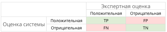

What are TP, TN, FP and some FN in this case?

In other words, we strive to ensure that the classifier's answers and the real state of affairs coincide. That is, to ensure that all numbers are distributed between the cells of TP and TN (true solutions) and do not fall into the FN and FP (false decisions).

And once we are talking about abbreviations, it's time to recall the accuracy metrics (Precision) and completeness (Recall).

If you deviate from the formal record, then Precision can be expressed as: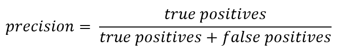

In other words, it is counted how many positive answers received from the classifier are correct. The greater the accuracy, the smaller the number of false hits (accuracy is 1 if there were no FPs).

Recall in its general form is presented as: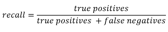

Recall characterizes the ability of the classifier to “guess” the largest possible number of positive answers from the expected ones. The higher the completeness, the less FN was.

Usually trying to balance between these two, but in this case, the priority will be fully given to Precision. The reason: a more humanistic approach, a desire to minimize the number of false-positive positives and, as a result, to avoid suspicion falling on the innocent.

We calculate Precision for our classifiers:

from sklearn.metrics import precision_score
defcalculate_precision(X, y):
    result = pd.DataFrame(columns=['classifier', 'precision'])
    for clf in classifiers:
        predicted = clf.predict(X_test)
        precision = precision_score(y_test, predicted, average='macro')
        classifier = clf.__class__.__name__
        classifier = classifier.replace('Classifier', '')
        result = result.append({'classifier': classifier, 'precision': precision}, ignore_index=True)
        print('Precision is {precision} for {classifier_name}'.format(precision=round(precision,2), classifier_name=classifier))
    result = result.sort_values(['classifier'], ascending=True)
    plt.subplots(figsize=(10, 7))
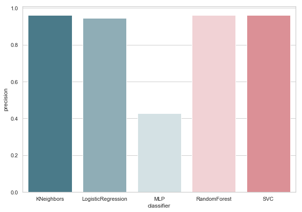
    sns.barplot(x="classifier", y='precision', palette=cmap, data=result)
calculate_precision(X_train, y_train)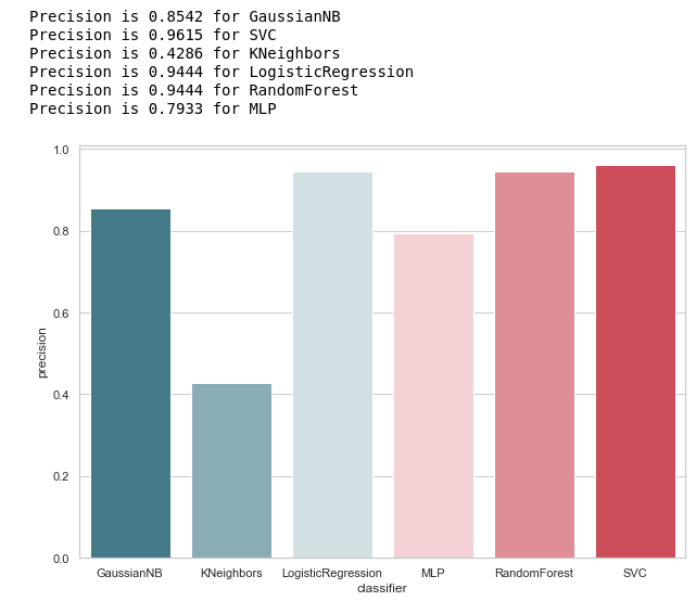

As follows from the figure, it turned out quite expectedly: the accuracy of KNeighbors turned out to be lower than everyone, because the value of TP is at its lowest.

At the same time, there is a good article on Habré about metrics, and those who want to dive deeper into this topic should read it.

Selection of hyper-parameters

After we have found the metric that best fits the selected conditions (we reduce the number of FPs), we can return to the first question: What is the reason for such behavior of the KNeighbors classifier?

The reason lies in the default parameters with which this model was created. And, most likely, to this stage, many could exclaim: why train on default parameters? There are special tools for the selection, for example, often used GridSearchCV.
Yes, it is, and it is time to resort to it,

But before that, we remove the Bayess classifier from our list. It allows one FP, and at the same time, this algorithm does not accept any variable parameters, as a result of which the result will not change.

classifiers.remove(gnb)

Adjustment

Let's set the parameter grid for each classifier:

parameters = {'SVC':{'kernel':('linear', 'rbf','poly'), 'C':[i for i in range(1,11)],'random_state': (random_state,)}, 
             'KNeighbors':{'algorithm':('ball_tree', 'kd_tree'), 'n_neighbors':[i for i in range(2,20)]},
             'LogisticRegression':{'penalty':('l1', 'l2'), 'C':[i for i in range(1,11)],'random_state': (random_state,)},
             'RandomForest':{'n_estimators':[i for i in range(10,101,10)],'random_state': (random_state,)},
             'MLP':{'activation':('relu','logistic'),'solver':('sgd','lbfgs'),'max_iter':(500,1000), 'hidden_layer_sizes':[(7,),(7,7)],'random_state': (random_state,)}}

Additionally, I wanted to draw attention to the number of layers / neurons in the MLP.
It was decided to set them not by enumerating all possible values, but still based on the formula :

I would like to say right away that training and cross-validation will be carried out only on the training set. I admit that there is an opinion that it is possible to do this on all data as in the example with Iris Dataset. But, in my opinion, such an approach is not entirely justified, since it will be impossible to trust the results of testing on a test sample.

We will optimize and replace our classifiers with their improved version:

from sklearn.model_selection import GridSearchCV
warnings.filterwarnings('ignore')
for idx,clf inenumerate(classifiers):
    classifier = clf.__class__.__name__
    classifier = classifier.replace('Classifier', '')
    params = parameters.get(classifier)
    if not params:
        continue
    new_clf = clf.__class__()
    gs = GridSearchCV(new_clf, params, cv=5)
    result =gs.fit(X_train, y_train)
    print(f'The best params for {classifier} are {result.best_params_}')
    classifiers[idx] = result.best_estimator_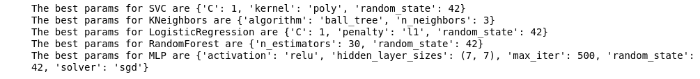

After we have selected the metric for evaluation and completed GridSearchCV, we are ready to draw the final line.

Summing up

Error Matrix v.2

matrices = make_confussion_matrices(X_train,y_train)
draw_confussion_matrices(1,2,first_row,figsize = (10.5,6))
draw_confussion_matrices(1,3,second_row,figsize = (16,6))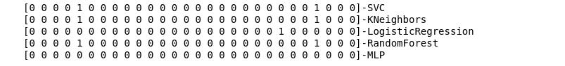

As can be seen from the matrix, the MLP showed degradation and considered that there were no suspects in the test sample. Random Forest added accuracy and corrected parameters for False Negative and True Positive. And KNeighbors showed an improvement in prediction. The forecast for others has not changed.

Accuracy v.2

Now, none of our current classifiers have errors with False Positive, which is good news. But, if we express everything in terms of numbers, we get the following picture:

calculate_precision(X_train, y_train)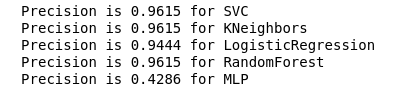 

Identified 3 classifier with the highest rate of precision. And they have the same values, based on the error matrix. Which classifier to choose?

Who is better?

It seems to me that this is a rather difficult question to which there is no universal answer. However, my point of view in this case would look something like this:

1. The classifier should be as simple in its technical implementation as possible. Then he will have less risk of retraining (this is probably what happened with the MLP). Therefore, it is not Random Forest, since this algorithm is an ensemble of 30 trees and, as a result, depends on them. In tune with one of the ideas of Python Zen: simple is better than complex.

2. Not bad when the algorithm was intuitive. That is, KNeighbors is perceived as simpler than SVM with potential multidimensional space.
Which in turn is similar to another statement: the explicit is better than the implicit.

Therefore, KNeighbors with 3 neighbors, in my opinion, the best candidate.

This is the end of the second part, which describes the use of Enron Dataset as an example of a classification task in machine learning. Based on materials from the course Introduction to Machine Learning at Udacity. There is also a python notebook , reflecting the entire sequence of actions described.