Hacker Guide to Neural Networks. Real Value Schemes. Strategy # 2: Numerical Gradient
- Transfer
Content:
We recall that at the beginning we had a scheme:
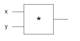
Our circuit has one logical element * and several defined initial values (for example, x = -2, y = 3). The logic element computes the result (-6) and we want to change x and y to make the result larger.
What we are going to do is as follows: Imagine that you took the output value, which is obtained from the circuit, and pull it in a positive direction. This positive tension will, in turn, be transmitted through the logic element and exert force on the initial values of x and y. Forces that tell us how x and y should change to increase the resulting value.
How such forces can look on our direct example? We can assume that the force exerted on x should also be positive, since a small increase in x improves the result of the circuit. For example, an increase from x = -2 to x = -1 will result in -3, which is much more than -6. On the other hand, a negative force should appear on y , which will cause it to decrease (since a lower value of y, for example, y = 2 , compared with the original y = 3 , will make the result higher: 2 x -2 = -4, which again is more than -6). In any case, this principle must be remembered. As we move on, it turns out that the forces that I described will actually be a derivative of the output values with respect to their original values (x and y). You have probably heard this term.
How can we really appreciate this power (derivative)? It turns out there is a fairly simple procedure for this. We will work in the opposite direction: instead of stretching the result of the circuit, we will change each initial value in turn, increase a little bit, and see what happens to the result. The number of changes in the output value is the derivative. But for now, enough theory. Let's look at a mathematical definition. We can write the derivative for our function with respect to the original values. For example, the derivative with respect to x can be calculated as follows:
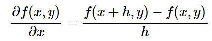
Where h is a small change value. In addition, if you are not particularly familiar with this calculation method, note that the horizontal line on the left side of the above equation does not mean division. The whole character (∂f (x, y)) / ∂x is a single element: the derivative of the function f (x, y) with respect to x. The horizontal line on the right is a division. I know this is complicated, but it is a standard notation. In any case, I hope this does not look too scary.
The circuit produced a certain initial result f (x, y), after which we changed one of the initial values to a small number h and got a new result f (x + h, y). Subtracting these two values shows us the change, and dividing by h simply leads the change to the (arbitrary) value of the change used by us. In other words, this expresses exactly what I described above and translates it into code like this:
recall that the forwardMultiplyGate (x, y) function returns the product of the arguments
Let's follow the example for x. We turned x into x + h, and the circuit responded with a higher value (again, note that -5.9997> -6). The division by h (in the derivative formula) is performed to bring the result of the circuit to the (arbitrary) value of h, which we decided to use in this case. Technically, we need h to be infinitesimal (an exact mathematical definition of the gradient is expressed as the limit of the expression as h tends to zero), but in practice h = 0.00001 or a similar value is perfect for most cases in which you need to get a good approximation. Now we see that the derivative with respect to x is +3. I specifically indicated the plus sign, as it shows that the circuit pulls x toward a higher value. The actual value of 3 can be interpreted as the force of such a tension.
By the way, we usually talk about the derivative with respect to one initial value, or about the gradient with respect to all such values. The gradient consists of the derivatives of all the original values connected in a vector (i.e. a list). Most importantly, if we allow the initial values to respond to the tension with a small value following the gradient (i.e., we add the derivative only to the top of each initial value), we can see that it increases, as we expected:
As expected, we changed the initial values to a gradient, and the circuit now produces a higher value (-5.87> -6.0). It was a lot easier than trying to arbitrarily change x and y, right? The fact is that if you perform the calculations, you can prove that the gradient is actually the direction of a sharp increase in the function. There is no need to dance with a tambourine, trying to substitute arbitrary values, as we did in strategy No. 1. To estimate the gradient, only three estimates of the circuit pass are required instead of hundreds, and we get the optimal push that we could count on (locally) if we are interested in increasing the output value.
More doesn't always mean better. Let me clarify a bit. Note that in this simplest example, using a step size (step_size) greater than 0.01 always gives the best result. For example, step_size = 1.0 results in -1 (bigger, better!), And a really infinite step size can give an infinitely good result. It is important to understand that as soon as our circuits become significantly more complex (for example, entire neural networks), functions from initial to output values will be more chaotic and “curly”. The gradient guarantees that if you have a very small (in fact, infinitesimal) step size, then you will definitely get a larger number if you follow in its direction, and for such an infinite small step size there is no other direction that would work just as well. But if you use a larger step (e.g. step_size = 0.01), everything will lose its meaning. The reason we can successfully use a larger step, instead of an infinite small one, is because our functions are usually relatively uniform. But in fact, we cross our fingers and hope for the best.
The analogy of climbing to the top. I once heard one analogy that the output value of our circuit is like the top of a hill, and we are trying to climb it blindfolded. We feel the steepness of the hillside under our feet (gradient), so if we move our legs a little bit, we will climb up. But if we take a big and too confident step, we can fall into the pit.
I hope I convinced you that a numerical gradient is really a very useful thing to evaluate, and also quite simple. But. It turns out that we can do even more, about which we will talk in the next part.
Chapter 1: Real Value Diagrams
Part 1:
Part 2:
Part 3:
Part 4:
Part 5:
Part 6:
   Введение
      Базовый сценарий: Простой логический элемент в схеме
      Цель
         Стратегия №1: Произвольный локальный поиск
Part 2:
Стратегия №2: Числовой градиент
Part 3:
Стратегия №3: Аналитический градиент
Part 4:
      Схемы с несколькими логическими элементами
         Обратное распространение ошибки
Part 5:
         Шаблоны в «обратном» потоке
      Пример "Один нейрон"
Part 6:
Становимся мастером обратного распространения ошибки
Chapter 2: Machine Learning
We recall that at the beginning we had a scheme:
Our circuit has one logical element * and several defined initial values (for example, x = -2, y = 3). The logic element computes the result (-6) and we want to change x and y to make the result larger.
What we are going to do is as follows: Imagine that you took the output value, which is obtained from the circuit, and pull it in a positive direction. This positive tension will, in turn, be transmitted through the logic element and exert force on the initial values of x and y. Forces that tell us how x and y should change to increase the resulting value.
How such forces can look on our direct example? We can assume that the force exerted on x should also be positive, since a small increase in x improves the result of the circuit. For example, an increase from x = -2 to x = -1 will result in -3, which is much more than -6. On the other hand, a negative force should appear on y , which will cause it to decrease (since a lower value of y, for example, y = 2 , compared with the original y = 3 , will make the result higher: 2 x -2 = -4, which again is more than -6). In any case, this principle must be remembered. As we move on, it turns out that the forces that I described will actually be a derivative of the output values with respect to their original values (x and y). You have probably heard this term.
The derivative can be considered as a force acting on each initial value as we increase the resulting value
How can we really appreciate this power (derivative)? It turns out there is a fairly simple procedure for this. We will work in the opposite direction: instead of stretching the result of the circuit, we will change each initial value in turn, increase a little bit, and see what happens to the result. The number of changes in the output value is the derivative. But for now, enough theory. Let's look at a mathematical definition. We can write the derivative for our function with respect to the original values. For example, the derivative with respect to x can be calculated as follows:
Where h is a small change value. In addition, if you are not particularly familiar with this calculation method, note that the horizontal line on the left side of the above equation does not mean division. The whole character (∂f (x, y)) / ∂x is a single element: the derivative of the function f (x, y) with respect to x. The horizontal line on the right is a division. I know this is complicated, but it is a standard notation. In any case, I hope this does not look too scary.
The circuit produced a certain initial result f (x, y), after which we changed one of the initial values to a small number h and got a new result f (x + h, y). Subtracting these two values shows us the change, and dividing by h simply leads the change to the (arbitrary) value of the change used by us. In other words, this expresses exactly what I described above and translates it into code like this:
recall that the forwardMultiplyGate (x, y) function returns the product of the arguments
var x = -2, y = 3;
var out = forwardMultiplyGate(x, y); // -6
var h = 0.0001;
// расчет производной по отношению к x
var xph = x + h; // -1.9999
var out2 = forwardMultiplyGate(xph, y); // -5.9997
var x_derivative = (out2 - out) / h; // 3.0
// расчет производной по отношению к y
var yph = y + h; // 3.0001
var out3 = forwardMultiplyGate(x, yph); // -6.0002
var y_derivative = (out3 - out) / h; // -2.0
Let's follow the example for x. We turned x into x + h, and the circuit responded with a higher value (again, note that -5.9997> -6). The division by h (in the derivative formula) is performed to bring the result of the circuit to the (arbitrary) value of h, which we decided to use in this case. Technically, we need h to be infinitesimal (an exact mathematical definition of the gradient is expressed as the limit of the expression as h tends to zero), but in practice h = 0.00001 or a similar value is perfect for most cases in which you need to get a good approximation. Now we see that the derivative with respect to x is +3. I specifically indicated the plus sign, as it shows that the circuit pulls x toward a higher value. The actual value of 3 can be interpreted as the force of such a tension.
The derivative with respect to any initial value can be calculated by adjusting this initial value to a small number and observing the change in the output value.
By the way, we usually talk about the derivative with respect to one initial value, or about the gradient with respect to all such values. The gradient consists of the derivatives of all the original values connected in a vector (i.e. a list). Most importantly, if we allow the initial values to respond to the tension with a small value following the gradient (i.e., we add the derivative only to the top of each initial value), we can see that it increases, as we expected:
var step_size = 0.01;
var out = forwardMultiplyGate(x, y); // раньше было: -6
x = x + step_size * x_derivative; // x становится -1.97
y = y + step_size * y_derivative; // y становится 2.98
var out_new = forwardMultiplyGate(x, y); // -5.87!
As expected, we changed the initial values to a gradient, and the circuit now produces a higher value (-5.87> -6.0). It was a lot easier than trying to arbitrarily change x and y, right? The fact is that if you perform the calculations, you can prove that the gradient is actually the direction of a sharp increase in the function. There is no need to dance with a tambourine, trying to substitute arbitrary values, as we did in strategy No. 1. To estimate the gradient, only three estimates of the circuit pass are required instead of hundreds, and we get the optimal push that we could count on (locally) if we are interested in increasing the output value.
More doesn't always mean better. Let me clarify a bit. Note that in this simplest example, using a step size (step_size) greater than 0.01 always gives the best result. For example, step_size = 1.0 results in -1 (bigger, better!), And a really infinite step size can give an infinitely good result. It is important to understand that as soon as our circuits become significantly more complex (for example, entire neural networks), functions from initial to output values will be more chaotic and “curly”. The gradient guarantees that if you have a very small (in fact, infinitesimal) step size, then you will definitely get a larger number if you follow in its direction, and for such an infinite small step size there is no other direction that would work just as well. But if you use a larger step (e.g. step_size = 0.01), everything will lose its meaning. The reason we can successfully use a larger step, instead of an infinite small one, is because our functions are usually relatively uniform. But in fact, we cross our fingers and hope for the best.
The analogy of climbing to the top. I once heard one analogy that the output value of our circuit is like the top of a hill, and we are trying to climb it blindfolded. We feel the steepness of the hillside under our feet (gradient), so if we move our legs a little bit, we will climb up. But if we take a big and too confident step, we can fall into the pit.
I hope I convinced you that a numerical gradient is really a very useful thing to evaluate, and also quite simple. But. It turns out that we can do even more, about which we will talk in the next part.