Probabilistic Models: Sampling
- Tutorial
Hello again! Today I continue the series of articles on the Surfingbird blog devoted to different methods of recommendations, and also sometimes just different kinds of probabilistic models. Long ago, it seems, last Friday in the summer of last year, I wrote a short cycle on graphical probabilistic models: the first part introduced the basics of graphical probabilistic models, in the second part there were several examples, part 3 talked about the message transfer algorithm, and in the fourth partWe briefly talked about variational approximations. The cycle ended with a promise to talk about sampling - well, not even a year has passed. Generally speaking, in this mini-cycle I will talk more specifically about the LDA model and how it helps us make recommendations for textual content. But today I will start by fulfilling a long-standing promise and telling about sampling in probabilistic models - one of the main methods of approximate inference.

First of all, I will remind you what we are talking about. One of the main tools of machine learning is the Bayes theorem:
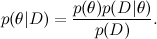
Here D is the data, θ are the parameters of the model that we want to train, and this is the distribution of θ subject to the available data D ; We have already spoken about Bayes' theorem in detail in one of the previous articles . In machine learning, we usually want to find a posterior distribution , and then predict new values of variables
  . In complex graphic models, all this, as we discussed in previous series, usually comes down to the fact that we have a large and confusing distribution of various random variables
 , which decomposes into a product of distributions more simply, and our task is to carry out marginalization , i.e. sum over part of variables or find the expectation of a function from part of variables. Note that all our problems somehow come down to calculating the mathematical expectation of different functions under the condition of a complex distribution, usually a conditional distribution of a model into which the values of some variables are substituted. We can also assume that we can count the value of the joint distribution at any point of it — this usually follows easily from the general form of the model, and the difficulty is to summarize and integrate over a bunch of these variables.
We already know that it is difficult to make an exact conclusion, and effective algorithms are obtained only for the case of a factor graph without cycles or with small cycles. However, real models often contain a bunch of variables that are closely related to each other and form a mass of cycles. We talked a little about variational approximations - one possible way to overcome the difficulties that arise. Today I’ll talk about another, even more popular method - about sampling.
The idea is simple to the extreme. We have already found out that, in principle, everything that we need is expressed in the form of expectations of various functions in our complex and confusing distribution p ( x ). How to calculate the expectation of a distribution function? If we can sample from this distribution, i.e. taking random points over the distribution of p ( x ), then the expectation of any function can be approximated as the arithmetic mean of the sampled points:

For example, to calculate the average (expectation), you need to average over the samples x .
Thus, our entire task actually comes down to learning how to sample points by distribution, provided that we can read the value of this distribution at any point.
It may seem to a person brought up on functions of one variable (i.e., practically to anyone who has attended the basic course of matanalysis at a university) that there is no big problem here, and all these conversations about anything - we know how to calculate the integral approximately, you just need to break the segment into pieces, calculate the function in the middle of each small segment, the rectangles there, the trapezoid, you know ... And really, there is nothing complicated in sampling from distributions from one variable. Difficulties, as always, begin with an increase in dimension - if in dimension 1 you need to count 10 values of the function to divide the interval into segments with side 0.1, then in dimension 100 such values will need 10 100which is much sadder. This and other effects, which make the work in high dimension completely unlike the usual 2-3 dimension, were called the curse of dimensionality; there are other interesting counterintuitive effects, maybe you should someday talk about this in more detail.
There is one more difficulty - I wrote above that we can read the distribution value at any point. Actually, in fact, we can consider not the distribution p ( x ), but the value of some function p * ( x ), which is proportional to p ( x) Remember Bayes' theorem - from it we get not the posterior distribution itself, but a function proportional to it:

Usually at this point we said that this is enough, and the exact value of the probability can simply be calculated by normalizing the resulting distribution so that it sums to unity (i.e. e. by computing the denominator in Bayes theorem). However, this is precisely the difficult task that we are now trying to learn how to solve: to summarize all the values of the complex distribution. Therefore, in real life, we cannot count on the value of true probabilities, only on some function p * proportional to them .
Despite all the above difficulties, sampling is still possible, and this is really one of the main methods of approximate output. Moreover, as we will soon see, sampling is not at all as difficult as it seems. In this section, I will talk about the basic idea on which all sampling algorithms are based in one way or another. The idea is this: if you evenly select a point under the graph of the distribution density function p , then its X-coordinate will be taken just from the distribution p . It is very easy to understand intuitively: imagine a density graph and break it into small columns, something like this (the graphs are made in matplotlib):
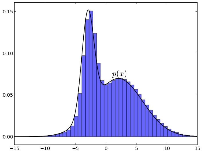
Now it’s clear that when you take a random point under the graph, each X-coordinate will meet with a probability proportional to the height of its column, i.e. Just with the value of the density function on this column.
Thus, we only need to learn how to take a random point under the density graph of the desired distribution. How to do this?
The first idea that really works and is often used in practice - the so-called sample with a deviation ( rejection sampling the ). Let's assume that we have some other distribution q (more precisely, the function q * proportional to it), which we already know how to sample. Usually this is some kind of classical distribution - uniform or normal. It is worth noting here that sampling from a normal distribution is also not a completely trivial task, but we will skip it now, for us now it’s enough to know that “people know how to do this”. Further, suppose that we know about him such a constant c that for all x . Then we can sample p in this way:
Here is a picture illustrating a sample with a deviation (normal distribution, chosen so as to majorize a mixture of two other Gaussians):
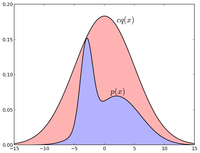
If the point under the graph cq * falls under the graph p * , i.e. into the blue zone, we take it; and if above it, i.e. into the red zone - we don’t take it. Again, it is easy to intuitively understand why this works: we take a random point uniformly under the cq * graph , and then leave only those points that fell under the p * graph at the same time - it is clear that in this case we will have just a uniform distribution under schedule p * . It is equally clear that if we can choose qquite similar to p (for example, we know roughly where p is concentrated and cover this area with a Gaussian), then this method will be much more effective than simply breaking up the entire space into identical pieces. But for the method to work, it is necessary that cq really approximates p quite well - if the area of the blue zone is 10 -10 of the area of red, no samples will work ...
There are different versions of this idea, which I will not dwell on in detail. In short, this idea and its variations work well with complex densities in units of units, but difficulties do begin in really high dimensions. Due to the effects of the dimensional curse, classical trial distributions of q get different unpleasant properties (for example, in a high dimension, the peel of an orange occupies almost its entire volume, and, in particular, the normal distribution is also almost entirely concentrated in a very thin “peel”, and not at all about zero), samples in the right places cannot be obtained, and the whole thing often fails. Need other methods.
The essence of this algorithm is based on the same idea: we want to take a point evenly under the function graph. However, the approach is now different: instead of trying to cover the entire distribution with a “cap” of the function q , we will act from the inside: we will build a random walkunder the function graph, moving from one point to another, and from time to time take the current wandering point as a sample. Since in this case this random walk is a Markov chain (i.e., its next point depends only on the previous one, and there is no memory), this class of algorithms is also called MCMC sampling (Markov chain Monte Carlo). To prove that the Metropolis-Hastings algorithm really works, you need to know the properties of Markov chains; but we’re not going to prove anything formally now, so I will just chastely leave a link to the wiki .
In fact, the algorithm is similar to the same sample with a deviation, but with an important difference: earlier, the distribution qwas common for the whole space, and now it will be local and will change over time, depending on the current point of wandering. As before, we consider a family of trial distributions , where
  is the current state. But now q should not be an approximation of p , but should just be some kind of sampled distribution that is concentrated in the vicinity of the current point - for example, a spherical Gaussian with a small dispersion is well suited. The candidate for the new state x 'will now be sampled from . The next iteration of the algorithm begins with the state and consists in the following:
The bottom line is that we move to a new distribution center if we take the next step, and we get a random walk depending on the distribution p : we always take a step if the density function increases in this direction, and sometimes we reject it if it decreases (we don't always reject , because we need to be able to get out of local maxima and wander under the whole graph p ). By the way, I note that when the step is rejected, we do not just discard a new point, but repeat the same x ( t ) a second time - thus, it is more likely to repeat samples around the local maxima of the distribution p , which corresponds to a higher density.
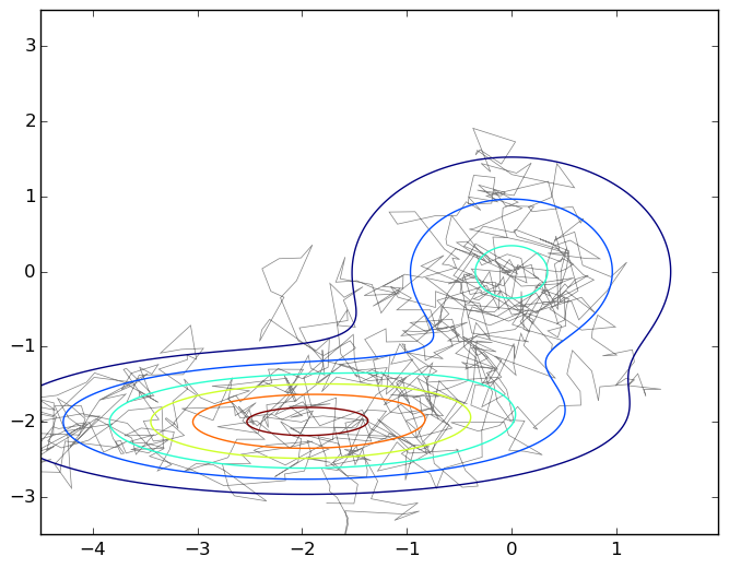
And again, the picture is a typical wandering on a plane under the graph of a mixture of two two-dimensional Gaussians:
To emphasize how simple this algorithm is, I will give the code that generated this graph.
So, we got a random walk under the density graph p ( x ); in fact, this still needs to be proved, but we won’t go into mathematics, so take a word. What now to do with this random walk, we need independent samples, and here it turns out that the next point of the walk certainly lies next to the previous one, and there is no trace of independence at all?
The answer is simple: you need to take not every point, but only some, separated from each other by many steps. Since this is a random walk, if most of q is concentrated in the radius ε, and the total radius in which p is concentrated is equal to D , then to obtain an independent sample, one will need steps. Again, you can take a word for it, or you can recall the classic problem from the course of probability theory about how far a point will go in n steps, which with equal probability moves left and right; it will go on average on
  , so it is logical that there will be a quadratic number of steps.
And now the main feature: this quadratic number depends on the radii of the two distributions, but it does not depend on the dimension at all . Monte Carlo Markov chain sampling is much less subject to a dimensional curse than the other methods we discussed; that is why it has become, one might say, the gold standard. In practice, however, Dit’s difficult to evaluate, so in specific implementations they usually do this: at first, a certain number of first steps, say 1000, are discarded (this is called a burn-in, and this is really important, because the starting point can fall into the unsuccessful region p , so before starting You need to make sure that we’ve walked long enough), and then each n- th sample is taken , where n is selected experimentally, based on the actual autocorrelation in the sequence of samples.
And the last sampling algorithm for today is Gibbs sampling. This is actually a special case of the Metropolis-Hastings algorithm, a very popular and simple special case.
The idea of sampling according to Gibbs is quite simple: suppose that we are in a very large dimension, the vector x is very long, and it is difficult for us to select the entire sample at once, it does not work. Let's try to choose a sample not all at once, but component wise. Then for sure these one-dimensional distributions will turn out to be simpler, and we will choose the sample.
Formally speaking, we run through the components of the vector, at each step we fix all the variables except one, and choose sequentially  according to the distribution

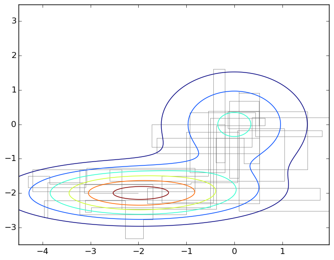
This differs from the general case of wandering around the Metropolis-Hastings in that now we move at each step along one of the coordinate axes; here is the corresponding picture:
Gibbs sampling is a special case of the Metropolis algorithm for distributions , and the probability of accepting each sample is always equal to 1 (you can prove this as an exercise). Therefore, the Gibbs sampling converges, and since this is the same random walk in fact, the same quadratic estimate is true.
No special assumptions or knowledge are needed for Gibbs sampling. You can quickly make a working model, and therefore it is a very popular algorithm. We also note that in large dimensions it may be more efficient to sample several variables at once rather than one at a time - for example, it often happens that we have a bipartite graph of variables in which all variables from one share are connected with all variables from another share (well or with many), but are not related to each other. In such a situation, God himself ordered to fix all the variables of one share and sample all the variables in another share at the same time (this can be taken literally - since with such a structure all the variables of one share are conditionally independent under the condition of another, they can be sampled independently and in parallel), then fix all second beat variables and so on.
Today we managed a lot: we talked about different sampling methods, which is one of the main tools for approximate inference in complex probabilistic models. Further I plan to develop this new mini-cycle towards thematic modeling, more precisely, the LDA model (latent Dirichlet allocation, latent Dirichlet allocation). In the next series, I will talk about the model itself (I briefly described it already , now you can talk in more detail) and explain how Gibbs sampling works for the LDA. And then we will gradually move on to how LDA and its many extensions for recommendation systems can be applied.
What is the task
First of all, I will remind you what we are talking about. One of the main tools of machine learning is the Bayes theorem:
Here D is the data, θ are the parameters of the model that we want to train, and
this is the distribution of θ subject to the available data D ; We have already spoken about Bayes' theorem in detail in one of the previous articles . In machine learning, we usually want to find a posterior distribution , and then predict new values of variables . In complex graphic models, all this, as we discussed in previous series, usually comes down to the fact that we have a large and confusing distribution of various random variables, which decomposes into a product of distributions more simply, and our task is to carry out marginalization , i.e. sum over part of variables or find the expectation of a function from part of variables. Note that all our problems somehow come down to calculating the mathematical expectation of different functions under the condition of a complex distribution, usually a conditional distribution of a model into which the values of some variables are substituted. We can also assume that we can count the value of the joint distribution at any point of it — this usually follows easily from the general form of the model, and the difficulty is to summarize and integrate over a bunch of these variables.We already know that it is difficult to make an exact conclusion, and effective algorithms are obtained only for the case of a factor graph without cycles or with small cycles. However, real models often contain a bunch of variables that are closely related to each other and form a mass of cycles. We talked a little about variational approximations - one possible way to overcome the difficulties that arise. Today I’ll talk about another, even more popular method - about sampling.
Monte Carlo Approach
The idea is simple to the extreme. We have already found out that, in principle, everything that we need is expressed in the form of expectations of various functions in our complex and confusing distribution p ( x ). How to calculate the expectation of a distribution function? If we can sample from this distribution, i.e. taking random points
over the distribution of p ( x ), then the expectation of any function can be approximated as the arithmetic mean of the sampled points: For example, to calculate the average (expectation), you need to average over the samples x .
Thus, our entire task actually comes down to learning how to sample points by distribution, provided that we can read the value of this distribution at any point.
What is the difficulty
It may seem to a person brought up on functions of one variable (i.e., practically to anyone who has attended the basic course of matanalysis at a university) that there is no big problem here, and all these conversations about anything - we know how to calculate the integral approximately, you just need to break the segment into pieces, calculate the function in the middle of each small segment, the rectangles there, the trapezoid, you know ... And really, there is nothing complicated in sampling from distributions from one variable. Difficulties, as always, begin with an increase in dimension - if in dimension 1 you need to count 10 values of the function to divide the interval into segments with side 0.1, then in dimension 100 such values will need 10 100which is much sadder. This and other effects, which make the work in high dimension completely unlike the usual 2-3 dimension, were called the curse of dimensionality; there are other interesting counterintuitive effects, maybe you should someday talk about this in more detail.
There is one more difficulty - I wrote above that we can read the distribution value at any point. Actually, in fact, we can consider not the distribution p ( x ), but the value of some function p * ( x ), which is proportional to p ( x) Remember Bayes' theorem - from it we get not the posterior distribution itself, but a function proportional to it:
Usually at this point we said that this is enough, and the exact value of the probability can simply be calculated by normalizing the resulting distribution so that it sums to unity (i.e. e. by computing the denominator in Bayes theorem). However, this is precisely the difficult task that we are now trying to learn how to solve: to summarize all the values of the complex distribution. Therefore, in real life, we cannot count on the value of true probabilities, only on some function p * proportional to them .
What to do: sample under the chart
Despite all the above difficulties, sampling is still possible, and this is really one of the main methods of approximate output. Moreover, as we will soon see, sampling is not at all as difficult as it seems. In this section, I will talk about the basic idea on which all sampling algorithms are based in one way or another. The idea is this: if you evenly select a point under the graph of the distribution density function p , then its X-coordinate will be taken just from the distribution p . It is very easy to understand intuitively: imagine a density graph and break it into small columns, something like this (the graphs are made in matplotlib):
Now it’s clear that when you take a random point under the graph, each X-coordinate will meet with a probability proportional to the height of its column, i.e. Just with the value of the density function on this column.
Thus, we only need to learn how to take a random point under the density graph of the desired distribution. How to do this?
The first idea that really works and is often used in practice - the so-called sample with a deviation ( rejection sampling the ). Let's assume that we have some other distribution q (more precisely, the function q * proportional to it), which we already know how to sample. Usually this is some kind of classical distribution - uniform or normal. It is worth noting here that sampling from a normal distribution is also not a completely trivial task, but we will skip it now, for us now it’s enough to know that “people know how to do this”. Further, suppose that we know about him such a constant c that for all x
. Then we can sample p in this way:- take the sample x on the distribution q * ( x );
- take a random number u uniformly from the interval
 ;
; - calculate p * ( x ); if it is greater than u , then x is added to the samples, and if it is less (i.e., if u did not fall under the density graph p * ), then x is rejected (hence the sample with a deviation).
Here is a picture illustrating a sample with a deviation (normal distribution, chosen so as to majorize a mixture of two other Gaussians):
If the point under the graph cq * falls under the graph p * , i.e. into the blue zone, we take it; and if above it, i.e. into the red zone - we don’t take it. Again, it is easy to intuitively understand why this works: we take a random point uniformly under the cq * graph , and then leave only those points that fell under the p * graph at the same time - it is clear that in this case we will have just a uniform distribution under schedule p * . It is equally clear that if we can choose qquite similar to p (for example, we know roughly where p is concentrated and cover this area with a Gaussian), then this method will be much more effective than simply breaking up the entire space into identical pieces. But for the method to work, it is necessary that cq really approximates p quite well - if the area of the blue zone is 10 -10 of the area of red, no samples will work ...
There are different versions of this idea, which I will not dwell on in detail. In short, this idea and its variations work well with complex densities in units of units, but difficulties do begin in really high dimensions. Due to the effects of the dimensional curse, classical trial distributions of q get different unpleasant properties (for example, in a high dimension, the peel of an orange occupies almost its entire volume, and, in particular, the normal distribution is also almost entirely concentrated in a very thin “peel”, and not at all about zero), samples in the right places cannot be obtained, and the whole thing often fails. Need other methods.
Metropolis-Hastings Algorithm
The essence of this algorithm is based on the same idea: we want to take a point evenly under the function graph. However, the approach is now different: instead of trying to cover the entire distribution with a “cap” of the function q , we will act from the inside: we will build a random walkunder the function graph, moving from one point to another, and from time to time take the current wandering point as a sample. Since in this case this random walk is a Markov chain (i.e., its next point depends only on the previous one, and there is no memory), this class of algorithms is also called MCMC sampling (Markov chain Monte Carlo). To prove that the Metropolis-Hastings algorithm really works, you need to know the properties of Markov chains; but we’re not going to prove anything formally now, so I will just chastely leave a link to the wiki .
In fact, the algorithm is similar to the same sample with a deviation, but with an important difference: earlier, the distribution qwas common for the whole space, and now it will be local and will change over time, depending on the current point of wandering. As before, we consider a family of trial distributions
, where is the current state. But now q should not be an approximation of p , but should just be some kind of sampled distribution that is concentrated in the vicinity of the current point - for example, a spherical Gaussian with a small dispersion is well suited. The candidate for the new state x 'will now be sampled from . The next iteration of the algorithm begins with the state and consists in the following:- select x 'by distribution ;
- calculate

(no need to be scared, for symmetric distributions, for example, a Gaussian, it is 1, this is just an asymmetry correction);
 - With probability a (1, if a > 1)
 , otherwise
  .
.
The bottom line is that we move to a new distribution center if we take the next step, and we get a random walk depending on the distribution p : we always take a step if the density function increases in this direction, and sometimes we reject it if it decreases (we don't always reject , because we need to be able to get out of local maxima and wander under the whole graph p ). By the way, I note that when the step is rejected, we do not just discard a new point, but repeat the same x ( t ) a second time - thus, it is more likely to repeat samples around the local maxima of the distribution p , which corresponds to a higher density.
And again, the picture is a typical wandering on a plane under the graph of a mixture of two two-dimensional Gaussians:
To emphasize how simple this algorithm is, I will give the code that generated this graph.
Python code
import numpy as np
import matplotlib.pyplot as plt
import matplotlib.patches as patches
import matplotlib.path as path
import matplotlib.mlab as mlab
import scipy.stats as stats
delta = 0.025
X, Y = np.meshgrid(np.arange(-4.5, 2.0, delta), np.arange(-3.5, 3.5, delta))
z1 = stats.multivariate_normal([0,0],[[1.0,0],[0,1.0]])
z2 = stats.multivariate_normal([-2,-2],[[1.5,0],[0,0.5]])
def z(x): return 0.4*z1.pdf(x) + 0.6*z2.pdf(x)
Z1 = mlab.bivariate_normal(X, Y, 1.0, 1.0, 0.0, 0.0)
Z2 = mlab.bivariate_normal(X, Y, 1.5, 0.5, -2, -2)
Z = 0.4*Z1 + 0.6*Z2
Q = stats.multivariate_normal([0,0],[[0.05,0],[0,0.05]])
r = [0,0]
samples = [r]
for i in range(0,1000):
	rq = Q.rvs() + r
	a = z(rq)/z(r)
	if np.random.binomial(1,min(a,1),1)[0] == 1:
		r = rq
		samples.append(r)
codes = np.ones(len(samples), int) * path.Path.LINETO
codes[0] = path.Path.MOVETO
p = path.Path(samples,codes)
fig, ax = plt.subplots()
ax.contour(X, Y, Z)
ax.add_patch(patches.PathPatch(p, facecolor='none', lw=0.5, edgecolor='gray'))
plt.show()
So, we got a random walk under the density graph p ( x ); in fact, this still needs to be proved, but we won’t go into mathematics, so take a word. What now to do with this random walk, we need independent samples, and here it turns out that the next point of the walk certainly lies next to the previous one, and there is no trace of independence at all?
The answer is simple: you need to take not every point, but only some, separated from each other by many steps. Since this is a random walk, if most of q is concentrated in the radius ε, and the total radius in which p is concentrated is equal to D , then to obtain an independent sample, one will need
steps. Again, you can take a word for it, or you can recall the classic problem from the course of probability theory about how far a point will go in n steps, which with equal probability moves left and right; it will go on average on , so it is logical that there will be a quadratic number of steps. And now the main feature: this quadratic number depends on the radii of the two distributions, but it does not depend on the dimension at all . Monte Carlo Markov chain sampling is much less subject to a dimensional curse than the other methods we discussed; that is why it has become, one might say, the gold standard. In practice, however, Dit’s difficult to evaluate, so in specific implementations they usually do this: at first, a certain number of first steps, say 1000, are discarded (this is called a burn-in, and this is really important, because the starting point can fall into the unsuccessful region p , so before starting You need to make sure that we’ve walked long enough), and then each n- th sample is taken , where n is selected experimentally, based on the actual autocorrelation in the sequence of samples.
Gibbs Sampling
And the last sampling algorithm for today is Gibbs sampling. This is actually a special case of the Metropolis-Hastings algorithm, a very popular and simple special case.
The idea of sampling according to Gibbs is quite simple: suppose that we are in a very large dimension, the vector x is very long, and it is difficult for us to select the entire sample at once, it does not work. Let's try to choose a sample not all at once, but component wise. Then for sure these one-dimensional distributions will turn out to be simpler, and we will choose the sample.
Formally speaking, we run through the components of the vector
, at each step we fix all the variables except one, and choose sequentially according to the distributionThis differs from the general case of wandering around the Metropolis-Hastings in that now we move at each step along one of the coordinate axes; here is the corresponding picture:
Gibbs sampling is a special case of the Metropolis algorithm for distributions
, and the probability of accepting each sample is always equal to 1 (you can prove this as an exercise). Therefore, the Gibbs sampling converges, and since this is the same random walk in fact, the same quadratic estimate is true.No special assumptions or knowledge are needed for Gibbs sampling. You can quickly make a working model, and therefore it is a very popular algorithm. We also note that in large dimensions it may be more efficient to sample several variables at once rather than one at a time - for example, it often happens that we have a bipartite graph of variables in which all variables from one share are connected with all variables from another share (well or with many), but are not related to each other. In such a situation, God himself ordered to fix all the variables of one share and sample all the variables in another share at the same time (this can be taken literally - since with such a structure all the variables of one share are conditionally independent under the condition of another, they can be sampled independently and in parallel), then fix all second beat variables and so on.
Conclusion
Today we managed a lot: we talked about different sampling methods, which is one of the main tools for approximate inference in complex probabilistic models. Further I plan to develop this new mini-cycle towards thematic modeling, more precisely, the LDA model (latent Dirichlet allocation, latent Dirichlet allocation). In the next series, I will talk about the model itself (I briefly described it already , now you can talk in more detail) and explain how Gibbs sampling works for the LDA. And then we will gradually move on to how LDA and its many extensions for recommendation systems can be applied.