Using the SQL query execution plan layer on VST diagrams
Performance optimization is an area in which everyone would like to become a great master. If we talk about experts in the field of working with databases, then we all come as newbies and at the beginning of our careers we spend a lot of time studying the basics, trying to understand the art of tuning database servers and applications to improve performance. However, and as you get deeper into the topic, optimizing performance doesn't get any easier.
With the development of technologies, the introduction of modern “flexible” approaches, and “continuous integration” in the field of databases, the need for a faster response to requests from end users only intensifies. In the current conditions of the spread of mobile devices, it is almost always required to make changes to data processing systems in order to accelerate the exchange of data with native or WEB-applications of users.
We are witnessing the constant emergence and introduction of new technologies. It's great! At the same time, the existing "old" technologies require a lot of attention and time to support. "Ocean" of data, "sea" of databases, more distributed systems. Less time is left for tuning and optimization. Reducing the windows for modifying, maintaining and making changes complicates the task of increasing the continuity of operation of systems on existing equipment.
In the field of tuning database optimization, there are often situations when it is difficult to choose the “right” solution. In such cases, you have to rely on various tools to help assess the situation and find ways to improve it. Having mastered such tools, it often becomes easier to find the best solution if a similar situation arises in the future.
In support of this thought, I will cite a translation of an interesting article from the bulldba.com/db-optimizer blog
Embarcadero's new DB Optimizer releases, starting with version 3.0, have a great new feature: overlay the explain plan with a query plan!
Take for example the following query:
Columns b.id and c.id create indexes. In the DB Optimizer window, this query looks like this:
Red lines of connections of this kind, according to the definitions, say that relationships can be many-to-many relationships.
Question: "What is the optimal execution plan for this request?"
One of the possible optimal execution plans for this “query tree” could be:
There is only one filter in this diagram. It is indicated by the green F symbol in table B. This table has a selection criterion “b.val2 = 100” in the query.
Ok, let's start with table B. Where do we go with our future implementation plan? Who is the "subordinate" and who is the "main"? How to determine? .. Oracle encounters the same difficulties in query planning. How to understand why Oracle made that decision and not the other? The new features of DB Optimizer come to the rescue here.
DB Optimizer has a super cool ability to overlay the current execution plan on the VST diagram (I like it so much!).
Now we see that Oracle starts with table B and connects it to table A. Is the result connected to table C. Is this plan optimal?
Leave the existing indexes and add a couple of constraints
Let us analyze the query in DB Optimizer again: Now we can see who is the main and who is the subordinate, based on this, determine the optimal plan for executing the query, which starts with filtering B, then connecting to C, then to A. Let's see how Oracle processes the added integrity constraints.
You see, the execution plan has changed in the light of constraints, and Oracle has moved the implementation plan from sub-optimal to optimal.
The moral of this story is that to be sure, you need to determine the integrity constraints in the database, because it contributes to the DBMS query optimizer, but the main thing I wanted to show here is an overlay of the query execution plan on the VST diagram, which makes a comparison of plans much simpler. Using the adjacent VST diagrams with superimposed query execution plans, you can quickly and easily see the differences.
I plan to write more about this feature. This is really great.
Here's another example from the Jonathan Lewis article www.simple-talk.com/sql/performance/designing-efficient-sql-a-visual-approach
In it, Jonathan discusses the request:
Which on the VST diagram looks like this:
There are several filters here, so we need to know which one is the most selective, so we’ll turn on the statistics on the diagram (the blue numbers below the tables are the percentage of filtering, green above the tables are the number of rows in the table , the numbers on the relationship lines represent the number of rows returned by the join of the two tables).
Now we can determine the best way to do the optimization. Did Oracle use it?
Could you see the optimizer error?
Dark green indicates the place where execution begins. Here, in two places: in the body of the main request and in the subquery. Red indicates the endpoint of the request.
Another example (Karl Arao):
Here, execution begins in 4 places. Notice how the result sets from each start are connected to each subsequent result of joining tables. The final is indicated in red.
[End of translation]
Optimization of database systems in modern environments often requires advanced knowledge, but, as before, for the most part remains an art.
Let's say it’s almost impossible for a person to test all valid options for hints and indexes to find the most optimal solution. You have to rely on smart tools like Embarcadero DB Optimizer, which will guide you through the setup process and help you choose the best option from the ones offered.
In the examples given, it was shown how its advanced capabilities helped not only quickly find the direction of query optimization, but also to get explanations for the decisions made by the “regular” Oracle optimizer, to find the missing descriptions that ensured a more “correct” work of the optimizer in the future.
For more information about working with VST diagrams, see the link to the article by Jonathan Lewis or on the Embarcadero website.
With the development of technologies, the introduction of modern “flexible” approaches, and “continuous integration” in the field of databases, the need for a faster response to requests from end users only intensifies. In the current conditions of the spread of mobile devices, it is almost always required to make changes to data processing systems in order to accelerate the exchange of data with native or WEB-applications of users.
We are witnessing the constant emergence and introduction of new technologies. It's great! At the same time, the existing "old" technologies require a lot of attention and time to support. "Ocean" of data, "sea" of databases, more distributed systems. Less time is left for tuning and optimization. Reducing the windows for modifying, maintaining and making changes complicates the task of increasing the continuity of operation of systems on existing equipment.
In the field of tuning database optimization, there are often situations when it is difficult to choose the “right” solution. In such cases, you have to rely on various tools to help assess the situation and find ways to improve it. Having mastered such tools, it often becomes easier to find the best solution if a similar situation arises in the future.
In support of this thought, I will cite a translation of an interesting article from the bulldba.com/db-optimizer blog
Embarcadero's new DB Optimizer releases, starting with version 3.0, have a great new feature: overlay the explain plan with a query plan!
[Translator’s Note:
Visual SQL Tuning (VST) optimization diagram turns SQL text into SQL graphical diagrams, shows indexes and constraints in tables and views using statistical information, and join operations used in SQL statements such as direct and implied Cartesian works and many-to-many relationships. ]
Take for example the following query:
SELECT COUNT (*)
FROM   a,  b,  c
WHERE
       b.val2 = 100 AND
       a.val1 = b.id AND
       b.val1 = c.id;
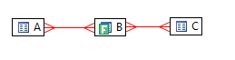
Columns b.id and c.id create indexes. In the DB Optimizer window, this query looks like this:
Red lines of connections of this kind, according to the definitions, say that relationships can be many-to-many relationships.
Question: "What is the optimal execution plan for this request?"
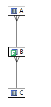
One of the possible optimal execution plans for this “query tree” could be:
- Start with the most selective filter.
- Run JOIN on subordinate tables if possible
- If not, then execute JOIN with the top level table
There is only one filter in this diagram. It is indicated by the green F symbol in table B. This table has a selection criterion “b.val2 = 100” in the query.
Ok, let's start with table B. Where do we go with our future implementation plan? Who is the "subordinate" and who is the "main"? How to determine? .. Oracle encounters the same difficulties in query planning. How to understand why Oracle made that decision and not the other? The new features of DB Optimizer come to the rescue here.
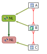
DB Optimizer has a super cool ability to overlay the current execution plan on the VST diagram (I like it so much!).
Now we see that Oracle starts with table B and connects it to table A. Is the result connected to table C. Is this plan optimal?
Leave the existing indexes and add a couple of constraints
alter table c add constraint c_pk_con unique (id);
alter table b add constraint b_pk_con unique (id);
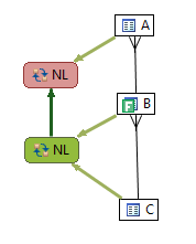
Let us analyze the query in DB Optimizer again: Now we can see who is the main and who is the subordinate, based on this, determine the optimal plan for executing the query, which starts with filtering B, then connecting to C, then to A. Let's see how Oracle processes the added integrity constraints.
You see, the execution plan has changed in the light of constraints, and Oracle has moved the implementation plan from sub-optimal to optimal.
The moral of this story is that to be sure, you need to determine the integrity constraints in the database, because it contributes to the DBMS query optimizer, but the main thing I wanted to show here is an overlay of the query execution plan on the VST diagram, which makes a comparison of plans much simpler. Using the adjacent VST diagrams with superimposed query execution plans, you can quickly and easily see the differences.
I plan to write more about this feature. This is really great.
Here's another example from the Jonathan Lewis article www.simple-talk.com/sql/performance/designing-efficient-sql-a-visual-approach
In it, Jonathan discusses the request:
SELECT order_line_data
FROM customers cus
         INNER JOIN
         orders ord
         ON ord.id_customer = cus.id
         INNER JOIN
         order_lines orl
         ON orl.id_order = ord.id
         INNER JOIN
         products prd1
         ON prd1.id = orl.id_product
         INNER JOIN
         suppliers sup1
         ON sup1.id = prd1.id_supplier
   WHERE
         cus.location = 'LONDON' AND
         ord.date_placed BETWEEN '04-JUN-10' AND '11-JUN-10' AND
         sup1.location = 'LEEDS' AND
    EXISTS (SELECT NULL
            FROM
                 alternatives alt
                 INNER JOIN
                 products prd2
                 ON prd2.id = alt.id_product_sub
                 INNER JOIN
                 suppliers sup2
                 ON sup2.id = prd2.id_supplier
           WHERE
                  alt.id_product = prd1.id AND
                  sup2.location != 'LEEDS')
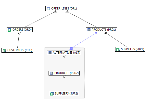
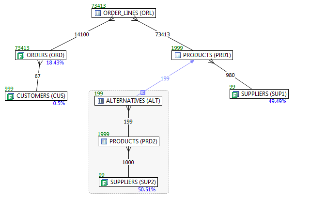
Which on the VST diagram looks like this:
There are several filters here, so we need to know which one is the most selective, so we’ll turn on the statistics on the diagram (the blue numbers below the tables are the percentage of filtering, green above the tables are the number of rows in the table , the numbers on the relationship lines represent the number of rows returned by the join of the two tables).
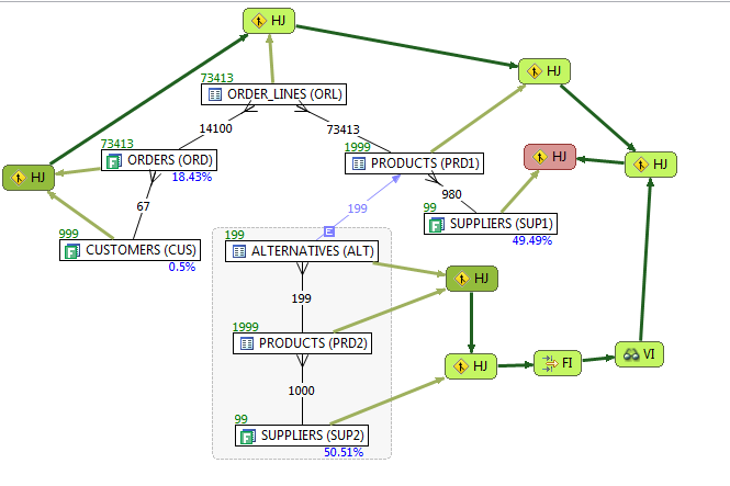
Now we can determine the best way to do the optimization. Did Oracle use it?
Could you see the optimizer error?
Dark green indicates the place where execution begins. Here, in two places: in the body of the main request and in the subquery. Red indicates the endpoint of the request.
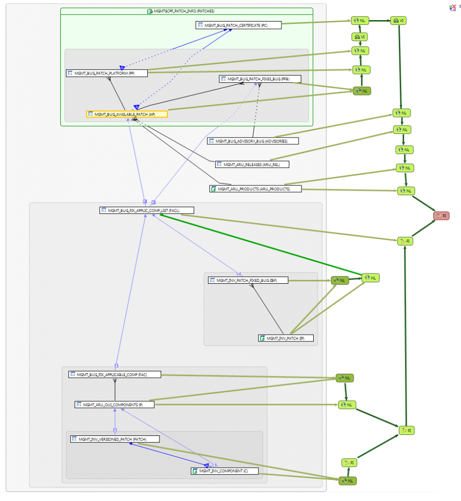
Another example (Karl Arao):
Here, execution begins in 4 places. Notice how the result sets from each start are connected to each subsequent result of joining tables. The final is indicated in red.
[End of translation]
Optimization of database systems in modern environments often requires advanced knowledge, but, as before, for the most part remains an art.
Let's say it’s almost impossible for a person to test all valid options for hints and indexes to find the most optimal solution. You have to rely on smart tools like Embarcadero DB Optimizer, which will guide you through the setup process and help you choose the best option from the ones offered.
In the examples given, it was shown how its advanced capabilities helped not only quickly find the direction of query optimization, but also to get explanations for the decisions made by the “regular” Oracle optimizer, to find the missing descriptions that ensured a more “correct” work of the optimizer in the future.
For more information about working with VST diagrams, see the link to the article by Jonathan Lewis or on the Embarcadero website.