Genetic algorithms in Matlab playfully

Foreword

Hello, Habr! I would like to offer you a simple applied lesson on genetic algorithms. If you are familiar and working with them, then reading it is a waste of time. This lesson is for those who want to start using, but don’t know how. It is assumed that you are already familiar with the meaning of genetic algorithms, have a little idea of ​​how they work.

The essence of genetic algorithms

Some may skip this part. Much has been said, I’ll just repeat it for order. Like any multivariate optimization algorithm, genetic algorithms are designed to minimize the objective function and produce a set of input arguments corresponding to a minimum. A pleasant feature of precisely genetic algorithms is the theoretical possibility of obtaining a global minimum of a function, read "getting the best possible answer." How this is achieved, I will explain a little later. Genetic algorithms, in essence, are nothing more than an approximate simulation of the evolutionary process. They operate with the concepts of "gene" and "population." A “gene” is a set of input arguments, and a “population” is a set of genes. In classical genetic algorithms, in order to obtain a gene from function arguments, they are simply written in a row in binary code. We get such a huge binary snake. As in the natural process of evolution, there is natural selection. Those genes for which the value of the function is the most eliminated, the best pass to the next generation without changes (elite). Others cross with other genes (cross-over). The method of crossing may be different. In the simplest case, each gene from an arbitrary pair is cut into two parts and the end of the second is attached to the beginning of the first gene, and the end of the first is attached to the beginning of the second. The proportions of the section, of course, should be equal for each of this pair. There is another, usually not numerous, group of mutant genes that randomly change one or more bits. It is they and the cross-over that provide the global minimum, even if we are in the local one. there is natural selection. Those genes for which the value of the function is the most eliminated, the best pass to the next generation without changes (elite). Others cross with other genes (cross-over). The method of crossing may be different. In the simplest case, each gene from an arbitrary pair is cut into two parts and the end of the second is attached to the beginning of the first gene, and the end of the first is attached to the beginning of the second. The proportions of the section, of course, should be equal for each of this pair. There is another, usually not numerous, group of mutant genes that randomly change one or more bits. It is they and the cross-over that provide the global minimum, even if we are in the local one. there is natural selection. Those genes for which the value of the function is the most eliminated, the best pass to the next generation without changes (elite). Others cross with other genes (cross-over). The method of crossing may be different. In the simplest case, each gene from an arbitrary pair is cut into two parts and the end of the second is attached to the beginning of the first gene, and the end of the first is attached to the beginning of the second. The proportions of the section, of course, should be equal for each of this pair. There is another, usually not numerous, group of mutant genes that randomly change one or more bits. It is they and the cross-over that provide the global minimum, even if we are in the local one. Others cross with other genes (cross-over). The method of crossing may be different. In the simplest case, each gene from an arbitrary pair is cut into two parts and the end of the second is attached to the beginning of the first gene, and the end of the first is attached to the beginning of the second. The proportions of the section, of course, should be equal for each of this pair. There is another, usually not numerous, group of mutant genes that randomly change one or more bits. It is they and the cross-over that provide the global minimum, even if we are in the local one. Others cross with other genes (cross-over). The method of crossing may be different. In the simplest case, each gene from an arbitrary pair is cut into two parts and the end of the second is attached to the beginning of the first gene, and the end of the first is attached to the beginning of the second. The proportions of the section, of course, should be equal for each of this pair. There is another, usually not numerous, group of mutant genes that randomly change one or more bits. It is they and the cross-over that provide the global minimum, even if we are in the local one. must be equal for each of this couple. There is another, usually not numerous, group of mutant genes that randomly change one or more bits. It is they and the cross-over that provide the global minimum, even if we are in the local one. must be equal for each of this couple. There is another, usually not numerous, group of mutant genes that randomly change one or more bits. It is they and the cross-over that provide the global minimum, even if we are in the local one.

Formulation of the problem

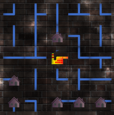
In the VK social network there is a rather interesting game called “Turn on the light”, it was she who aroused the desire to write an article, since the tasks that the user solves in it are just great for genetic algorithms. In three words, the essence of the game is as follows: it is necessary to connect the power station and the houses with cables. On each cell of the playing field there is one of four types of cables: L-shaped, T-shaped, I-shaped, half of the I-shaped for connecting the house (denoted by H). The player is free to rotate them in increments of 90 degrees. In general, at first it is better to try to understand.
Have you tried it? Move on. It is necessary to build the objective function of the state of the playing field. The input data is the rotation angle of each of the cable fragments. It is easy to understand that it can be encoded in 2 bits. The total field at the beginning of the game is 5x5 squares. Therefore, the length of the gene in binary code is 5x5x2 = 50 bits. The objective function will accept an array of zeros and ones as input (in Matlab there is such a possibility).
How to evaluate the quality of the state of the playing field? I suggest using the number of connections between neighboring cells. The score of the playing field is the sum of the ratings of the cells. Each cell connection with a neighbor is a score. Neighbors in cells 4: upper, lower, left, right.

Implementation Features

I would not want to paste the sources and disassemble them line by line, as some people like to do on Habré. The git repository will do just that: github.com/player999/turnonthelight . Comments in README should help. Now I advise you to open the source and copy them along with the article. I purposely made them simpler enough. Just touch on the important points of implementation. At the input of the program, the initial state of the playing field in a text file is approximately in the following form:

H1 H0 I1 I1 I3
I1 H2 T1 T1 I3
L3 L2 H1 L0 H1
H0 L1 T3 I0 T3
L0 I0 L0 L0 L0

Here the letter is the type of cell, and the number is the orientation from 0 to 270 degrees in increments of 90 degrees clockwise. This field is read using the scheme_config function, which is called from the main run script. Further, a genetic algorithm can be applied to it by calling the solve_scheme function. In the run script, the target function is designated as fun, which is a wrapper for the eval_bits function. eval_bits accepts two binary strings that describe the playing field. The first is the cell types, the second is their orientation. Naturally, during the operation of the genetic algorithm, the first parameter must be constant. The player cannot change cell types. These lines are constructed of the array of cells of the playing field with the scheme2string function. eval_bits is a wrapper for eval_scheme. This is the core of the objective function, and eval_bits simply converts the arguments into a matrix,
I hope it is clear how the objective function works. Now to the very minimization. First you need to get a structure with options for the genetic algorithm. There are many for every taste. But indicated only the most important. PopulationType - presentation of arguments. In our case, a bit string. And although the word "string" appears here, in fact it is a double array of zeros and ones. PopulationSize - how many genes will be in each iteration. The more genes, the better the algorithm will work, but at the same time it will be slower. For each buck gene, you need to calculate the objective function. Generations - the number of iterations of the genetic algorithm. This is one of the possible exit conditions. Another, for example, is the way out when the change in the objective function stops.
options = gaoptimset('PopulationType','bitstring','PopulationSize',1000,'Generations',100);




The optimization function call follows: Arrays with restrictions are skipped here, since they are not relevant for this task. length (pos) reflects the number of arguments. You can read more about these functions in the help of Matlab, it is gorgeous. I also recommend playing with the Optimization Toolbox settings (optimtool command), all the same settings, dressed in a graphical interface for convenience. Next, the best gene is converted using string2scheme back to the playing field and the game field is drawn with the draw_scheme function.
opt = ga(fun,length(pos),[],[],[],[],[],[],[],options);


conclusions

Although the algorithm also requires customization, it confidently proved that it can search for solutions to the puzzle. I hope the article helped you a little, or at least entertained you. Here is the result of the work, for example.