Draw a map with one select or about the benefits of multi-table indexes
This article was written in the continuation of a series that describes the prototyping of a simple and productive dynamic web map server. Earlier it was told how spatial indexes are arranged in it, as well as how you can just take and draw a spatial layer. Now we will do it a little more elegant.
As for working with one layer, we more or less figured out, but in reality there can be dozens of layers, each of them will have to be requested in the spatial index, even if nothing got into the search extent ... Is it possible somehow to architecturally clean this process and get rid of obviously useless actions?
Indexing
It’s possible, why not. But for this we will have to create a single spatial index for all spatial layers. Recall how our indexes are structured:
- The layer space is divided into rectangular blocks
- All blocks are numbered.
- Each indexed object is assigned one or more block numbers in which it is located
- When searching, the extent of the query is split into blocks, and for each block or a continuous chain of blocks from a regular integer index, all objects that belong to them are obtained
Well, to create a single index, you will have to divide all the layers with one grid, number the blocks the same way, and in addition to the object identifier, store the table identifier in the index. So:
- We will train as before on the shape data obtained from OSM Russia .
- Take 4 relatively populated layers - ponds, forests, buildings and roads.
- As before, we will use the OpenSource edition of OpenLink Virtuoso , the official Win_x64 build of version 7.0.0, taken from the developer's site, as before.
- For drawing, we will use a GD- based and previously described C plugin that extends the set of built-in PL / SQL functions.
- We take the data extent: xmin = -180, ymin = 35, xmax = 180, ymax = 85 degrees.
- We divide this extent into blocks of 0.1 ° in latitude and longitude. Thus we get a grid of 3600X500 blocks. 0.1 ° is about 11 km, a bit much for drawing at the level of houses, but our goal at the moment is not maximum performance in specific conditions, but a concept check.
- We load the layers in the DBMS as before:
- vegetation-polygon.shp: 657673 elements, load time 2 '4' '
- water-polygon.shp: 380868 elements, load time 1 '22' '
- building-polygon.shp: 5326421 elements, load time 15 '42' '
- highway-line.shp: 2599083 elements, load time 7 '56' '
- Now there are tables with data (Ex: "xxx". "YYY". "Water-polygon") and related tables with spatial indexes (Ex: "xxx". "YYY". "Water-polygon__spx"). Taking advantage of the fact that they are all formed with the same parameters, we merge them in a single spatial index
Making a general index takes 2'16 ''. Using cursors instead of constructs (insert ... select ...) is caused by the fact that in the OpenSource version there is a limit of 50mb on the size of the log of one transaction in the log. This restriction is easy to remove by rebuilding, but that's another story.registry_set ('__spx_startx', '-180'); registry_set ('__spx_starty', '35'); registry_set ('__spx_nx', '3600'); registry_set ('__spx_ny', '500'); registry_set ('__spx_stepx', '0.1'); registry_set ('__spx_stepy', '0.1'); drop table "xxx"."YYY"."total__spx"; create table "xxx"."YYY"."total__spx" ( "node_" integer, "tab_" integer, "oid_" integer, primary key ("node_", "tab_", "oid_")); create procedure mp_total_spx () { for select "node_", "oid_" from "xxx"."YYY"."water-polygon__spx" do { insert into "xxx"."YYY"."total__spx" ("oid_","tab_","node_") values ("oid_", 1, "node_"); commit work; } for select "node_", "oid_" from "xxx"."YYY"."vegetation-polygon__spx" do { insert into "xxx"."YYY"."total__spx" ("oid_","tab_","node_") values ("oid_", 2, "node_"); commit work; } for select "node_", "oid_" from "xxx"."YYY"."highway-line__spx" do { insert into "xxx"."YYY"."total__spx" ("oid_","tab_","node_") values ("oid_", 3, "node_"); commit work; } for select "node_", "oid_" from "xxx"."YYY"."building-polygon__spx" do { insert into "xxx"."YYY"."total__spx" ("oid_","tab_","node_") values ("oid_", 4, "node_"); commit work; } }; mp_total_spx (); - Now we set up working with the index in the same way as we did before
create procedure "xxx"."YYY"."total__spx_enum_items_in_box" ( in minx double precision, in miny double precision, in maxx double precision, in maxy double precision) { declare nx, ny integer; nx := atoi (registry_get ('__spx_nx')); ny := atoi (registry_get ('__spx_ny')); declare startx, starty double precision; startx := atof (registry_get ('__spx_startx')); starty := atof (registry_get ('__spx_starty')); declare stepx, stepy double precision; stepx := atof (registry_get ('__spx_stepx')); stepy := atof (registry_get ('__spx_stepy')); declare sx, sy, fx, fy integer; sx := cast (floor ((minx - startx)/stepx) as integer); fx := cast (floor ((maxx - startx)/stepx) as integer); sy := cast (floor ((miny - starty)/stepy) as integer); fy := cast (floor ((maxy - starty)/stepy) as integer); declare ress any; ress := vector(dict_new (), dict_new (), dict_new (), dict_new ()); for (declare iy integer, iy := sy; iy <= fy; iy := iy + 1) { declare ixf, ixt integer; ixf := nx * iy + sx; ixt := nx * iy + fx; for select "node_", "tab_", "oid_" from "xxx"."YYY"."total__spx" where "node_" >= ixf and "node_" <= ixt do { dict_put (ress["tab_" - 1], "oid_", 0); } } result_names('oid', 'tab'); declare ix integer; for (ix := 0; ix < 4; ix := ix + 1) { declare arr any; arr := dict_list_keys (ress[ix], 1); gvector_digit_sort (arr, 1, 0, 1); foreach (integer oid in arr) do { result (oid, ix + 1); } } }; create procedure view "xxx"."YYY"."v_total__spx_enum_items_in_box" as "xxx"."YYY"."total__spx_enum_items_in_box" (minx, miny, maxx, maxy) ("oid" integer, "tab" integer); - Check the correct operation:
The first request returned 29158, the rest: 941 + 33 + 20131 + 8053. Matches.select count(*) from "xxx"."YYY"."v_total__spx_enum_items_in_box" as a where a.minx = 82.963 and a.miny = 54.9866 and a.maxx = 82.98997 and a.maxy = 55.0133; select count(*) from "xxx"."YYY"."v_vegetation-polygon_spx_enum_items_in_box" ... select count(*) from "xxx"."YYY"."v_water-polygon_spx_enum_items_in_box" ... select count(*) from "xxx"."YYY"."v_building-polygon_spx_enum_items_in_box" ... select count(*) from "xxx"."YYY"."v_highway-line_spx_enum_items_in_box" ...
Measure the performance of the index.
We will run a series of 10,000 random searches in the square [35 ... 45.50 ... 60] ° on the general index and in the old way. All requests are executed in one connection i.e. show performance on a single core.
| Request Size | Time in a single index | Old time |
|---|---|---|
| 0.01 ° | 7'35 '' | 8'26 '' |
| 0.1 ° | 8'25 '' | 9'20 '' |
| 0.5 ° | 15'11 '' | 16'7 '' |
Draw a map
First of all, we will draw it in the old way , so that there is something to compare.
create procedure mk_test_gif(
	in cminx double precision,
	in cminy double precision,
	in cmaxx double precision,
	in cmaxy double precision)
{
  declare img any;
  img := img_create (512, 512, cminx, cminy, cmaxx, cmaxy, 1);
  declare cl integer;
  declare bg integer;
  {
    cl := img_alloc_color (img, 0, 0, 255);
    bg := img_alloc_color (img, 0, 0, 255);
    whenever not found goto nf;
    for select blob_to_string(Shape) as data from
      xxx.YYY."water-polygon" as x, xxx.YYY."v_water-polygon_spx_enum_items_in_box" as a
    where a.minx = cminx and a.miny = cminy and a.maxx = cmaxx and a.maxy = cmaxy
      and x."_OBJECTID_" = a.oid
      and x.maxx_ >= cminx and x.minx_ <= cmaxx
      and x.maxy_ >= cminy and x.miny_ <= cmaxy
    do  { img_draw_polygone (img, data, cl, bg); }
nf:;
...
  для остальных таблиц примерно то же, дороги рисуются через img_draw_polyline.
...
  }
  declare ptr integer;
  ptr := img_tostr (img);
  img_destroy (img);
  declare image any;
  image := img_fromptr(ptr);
  string_to_file('test.gif', image, -2);
  return;
};
mk_test_gif(35., 50., 45., 60.);
Now, as promised, in one select. The first thing that comes to mind is
aggregates .
An aggregate is an object that is created when the cursor is opened, called on each line of the result, and finalized when the cursor is closed.
create function mapx_agg_init (inout _agg any)
{;};
create function mapx_agg_acc (
  inout _agg any,
  in _tab integer,
  in _oid integer )
{
  if (_agg is null)  {
    declare img any;
    img := img_create (512, 512, _tab[0], _tab[1], _tab[2], _tab[3], 1);
    _agg := img;
    return 0;
  }  else  {
    return case
      when _tab = 4 then (img_draw_polygone(_agg, (
        select blob_to_string(bl.Shape) from "xxx"."YYY"."building-polygon" as bl
        where bl."_OBJECTID_" = _oid), 255, 255))
      when _tab = 3 then (img_draw_polyline(_agg, (
        select blob_to_string(hw.Shape) from "xxx"."YYY"."highway-line" as hw
        where hw."_OBJECTID_" = _oid), 100, 100))
      when _tab = 2 then (img_draw_polygone(_agg, (
        select blob_to_string(vg.Shape) from "xxx"."YYY"."vegetation-polygon" as vg
        where vg."_OBJECTID_" = _oid), 10, 10))
      when _tab = 1 then (img_draw_polygone(_agg, (
        select blob_to_string(wt.Shape) from "xxx"."YYY"."water-polygon" as wt
        where wt."_OBJECTID_" = _oid), 50, 50))
      else 1
    end;
  }
};
create function mapx_agg_final (inout _agg any) returns integer
{
  declare ptr integer;
  ptr := img_tostr (_agg);
  img_destroy (_agg);
  declare image any;
  image := img_fromptr(ptr);
  string_to_file('nskx_ii.gif', image, -2);
  return 1;
};
create aggregate mapx_agg (in _tab integer, in _oid integer) returns integer
  from mapx_agg_init, mapx_agg_acc, mapx_agg_final;
create procedure mk_testx_ii_gif(
	in cminx double precision,
	in cminy double precision,
	in cmaxx double precision,
	in cmaxy double precision)
{
  declare cnt integer;
  select
      mapx_agg(tab, oid) into cnt
  from (
    select * from (select vector(cminx, cminy, cmaxx, cmaxy) as tab, 0 as oid) as f1
    union all
    (select tab, oid from xxx.YYY."v_total__spx_enum_items_in_box" as a
     where a.minx = cminx and a.miny = cminy and a.maxx = cmaxx and a.maxy = cmaxy)
  ) f_all;
}
mk_testx_ii_gif(35., 50., 45., 60.);
How can it be, an attentive reader will say, one select was promised, and there are a whole bunch of them! Actually, the row identifiers come to the aggregate in an orderly and tabular manner, so the apparent subqueries are actually organized by join hands.
So, the run time is 42 seconds. Nda.
Another attempt
create procedure mk_testx_gif(
	in cminx double precision,
	in cminy double precision,
	in cmaxx double precision,
	in cmaxy double precision)
{
  declare img any;
  img := img_create (512, 512, cminx, cminy, cmaxx, cmaxy, 1);
  declare cnt, cnt2 integer;
  declare cl1, bg1 integer;
  cl1 := img_alloc_color (img, 0, 0, 255);
  bg1 := img_alloc_color (img, 0, 0, 255);
  declare cl2, bg2 integer;
  cl2 := img_alloc_color (img, 0, 255, 0);
  bg2 := img_alloc_color (img, 0, 255, 0);
  declare cl3, bg3 integer;
  cl3 := img_alloc_color (img, 255, 100, 0);
  bg3 := img_alloc_color (img, 255, 100, 0);
  declare cl4, bg4 integer;
  cl4 := img_alloc_color (img, 255, 0, 0);
  bg4 := img_alloc_color (img, 255, 0, 0);
  select
    sum (
      case
        when geom is null then 0
        when geom_type = 2 then (img_draw_polyline(img, geom, cl, bg))
        else (img_draw_polygone(img, geom, cl, bg))
      end
    ) into cnt
  from (
    select
      case
        when a.tab = 4 then (
           select blob_to_string(bl.Shape) from "xxx"."YYY"."building-polygon" as bl
           where bl."_OBJECTID_" = a.oid)
        when a.tab = 3 then (
           select blob_to_string(hw.Shape) from "xxx"."YYY"."highway-line" as hw
           where hw."_OBJECTID_" = a.oid)
        when a.tab = 2 then (
           select blob_to_string(vg.Shape) from "xxx"."YYY"."vegetation-polygon" as vg
           where vg."_OBJECTID_" = a.oid)
        when a.tab = 1 then (
           select blob_to_string(wt.Shape) from "xxx"."YYY"."water-polygon" as wt
           where wt."_OBJECTID_" = a.oid)
        else ''
      end as geom,
      case when a.tab = 3 then 2 else 1 end as geom_type,
      case when a.tab = 4 then cl4
           when a.tab = 3 then cl3
           when a.tab = 2 then cl2
           when a.tab = 1 then cl1 else 0 end as cl,
      case when a.tab = 4 then bg4
           when a.tab = 3 then bg3
           when a.tab = 2 then bg2
           when a.tab = 1 then bg1 else 0 end as bg
    from
      xxx.YYY."v_total__spx_enum_items_in_box" as a
    where a.minx = cminx and a.miny = cminy
           and a.maxx = cmaxx and a.maxy = cmaxy
  ) f_all;
  declare ptr integer;
  ptr := img_tostr (img);
  img_destroy (img);
  declare image any;
  image := img_fromptr(ptr);
  string_to_file('testx.gif', image, -2);
  return;
};
mk_testx_gif(35., 50., 45., 60.);
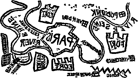
And here is the result:
There are several million objects in this nondescript picture.
conclusions
Draw a map with one request is not difficult. We even managed to do this without losing much in performance. True, it also failed to win, and the reason seems to be in the data structure. And this structure is sharpened for use by traditional GIS.
For example, the table 'highway-line' contains a couple of dozens of layers of different types that differ in attributes. Usually, such tables serve as the basis for all road layers that refer to one physical table and differ in filters. Of course, it is more convenient to work with one table than with two dozen (this point was also one of the motives for this work). Again, we have a common spatial index for all of these layers.
But there are also disadvantages. Still, to draw each layer, you need to run a separate SQL query. Those. even though there’s one index, there’s still a few searches on it. The most you can win on is caching pages. An additional index is needed - the type of record; it is also required to search on it and cross the samples. In addition, since objects of different types are mixed up, there is little chance that objects of the same type will appear side by side (on the same page) and thereby increase the total number of readings.
What if, for example, we scatter the 'highway-line' table into a bunch of sub-tables by type and combine all of them in one spatial index, as we did above? Working with the index will not change from this, we will need only one search in it. Work with data will only accelerate since the locality of the data will increase - data of the same type, close spatially more often will be next to the disk. And if any type of data is not in the search extent, it simply will not be processed. No matter how many there are, this will not affect the reading of useful data.
And one last observation. Indexes as such are rather strange objects. Neither in relational algebra, nor in relational calculus are they even close. This is an implementation-specific extension that allows the query processor to execute them more efficiently. In our case, the indices are loaded with some semantics that are not in the data. Our multi-table index describes the relationships between layers, in fact, in a particular index are those layers that we want to draw together.
On the other hand, we cannot perceive our index as a table (although in fact it is a table, this is a necessary measure due to the fact that we are forced to remain within a specific DBMS) because its values are table identifiers. This is a metatable and the query plan depends on the metadata from this one.
Again, traditionally, the query processor is free to choose which indexes to use for it. But this is not our case. We can create several multi-table indexes and explicitly indicate which index is the source of the primary data stream. Regardless of what the optimizer thinks about this. It’s nice to see how the “tree of life is always green” through the “dry theory” of the relational model.