Anatomy of recommender systems. Part two
A week ago, I reviewed the existing recommendation algorithms here . In this article I will continue this review: I’ll talk about the item-based version of collaborative filtering, methods based on matrix expansions, testing problems, as well as less-promoted (but equally interesting) algorithms.

The Item-based approach is a natural alternative to the classic User-based approach, described in the first part, and almost repeats it, except for one thing - it applies to the transposed preference matrix. Those. looking for close products, not users.
Let me remind you, user-based CF (user-based CF) searches for each client a group of the most similar to it (in terms of previous purchases) customers and averages their preferences. These average preferences serve as recommendations for the user. In the case of commodity-based collaborative filtering (item-based CF), the nearest neighbors are searched for on a variety of products — columns of a preference matrix. And the averaging occurs exactly according to them.
Indeed, if the products are meaningfully similar, then most likely they either at the same time like them or at the same time dislike them. Therefore, when we see that the two products have a strong correlation between the estimates, this may indicate that these are equivalent products.
Advantages of Item-based over User-based:
The rest of the algorithm almost completely repeats the User-based version: the same cosine distance as the main measure of proximity, the same need for data normalization. The number of neighboring goods N is usually chosen in the region of 20.
Due to the fact that the correlation of products is considered on a larger number of observations, it is not so critical to recalculate it after each new assessment and this can be done periodically in batche mode.
Several possible improvements to the algorithm:
When using the item-based approach, recommendations tend to be more conservative. Indeed, the spread of recommendations is less and therefore less likely to show non-standard products.
If in the matrix of preferences we use the review of the description of the product as a rating, then the recommended products will most likely be analogues - products that are often viewed together. If the ratings in the matrix of preferences, we expect on the basis of purchases, then most likely the recommended products will be accessories - products that are often bought together.
Testing a recommender system is a difficult process and always causing many questions, mainly due to the ambiguity of the very concept of “quality”.
In general, in problems of machine learning there are two main approaches to testing:
Both of these approaches are actively used in the development of recommender systems. Let's start with offline testing.
The main constraint that we face is that we can assess the accuracy of the forecast only on those products that the user has already rated.
The standard approach is cross-validation with the leave-one-out and leave-p-out methods. Multiple repetition of the test with averaging results provides a more stable assessment of quality.
All quality metrics can be divided into three categories:
Unfortunately, there is no single recommended metric for all occasions, and everyone who is involved in testing a recommender system selects it to fit its goals.
When ratings are rated on a continuous scale (0-10), as a rule, Prediction Accuracy class metrics are sufficient.
Decision Support class metrics work with binary data (0 and 1, yes and no). If, in our problem, the ratings are initially set aside on a continuous scale, they can be converted to a binary format by applying the decision rule - say, if the score is less than 3.5, we consider the mark as “bad”, and if it is greater, then “good”.
As a rule, recommendations are displayed in a list of several positions (first, top one, then in descending order of priority). Rank Accuracy class metrics measure how correct the order of recommendations in a sorted list is.
If we take recommender systems in online business, then they, as a rule, pursue two (sometimes contradictory) goals:
As in any model aimed at motivating the user to action, only incremental increment of the target action should be evaluated. Ie, for example, when calculating purchases on the recommendation, we need to exclude those that the user himself would have done without our model. If this is not done, the effect of the introduction of the model will be greatly overestimated.
Lift is an indicator of how many times the accuracy of a model exceeds a certain baseline algorithm. In our case, the baseline algorithm may simply be the lack of recommendations. This metric well captures the share of incremental purchases and this allows you to effectively compare different models.
 Source
User behavior is a thing that is poorly formalized and not a single metric will fully describe the thought processes in his head when choosing a product. Many factors affect the decision. Follow the link with the recommended product is not yet its high score or even interest. Partially understand the logic of the client helps online testing. Below are a couple of scenarios for such testing.
The first and most obvious scenario is the analysis of site events. We look at what the user does on the site, whether he pays attention to our recommendations, whether he follows them, which features of the system are in demand, which are not, which products are better recommended, and which are worse. To understand which of the algorithms as a whole works better or just try a new promising idea, we do A / B testing and collect the result.
The second scenario is receiving feedback from users in the form of polls and polls. As a rule, these are general questions for understanding how customers use the service — which is more important: relevance or diversity, is it possible to show duplicate products, or is it too annoying. The advantage of the script is that it gives a direct answer to all these questions.
Such testing is difficult, but for large reference services, it is simply necessary. Questions may be more complex, for example, “which of the lists seems to be more relevant to you,” “how much the sheet looks solid,” “whether you will watch this film / read a book”.
At the beginning of its development, recommender systems were used in services where the user explicitly assesses the product by rating him — this is Amazon, Netflix, and other Internet commerce sites. However, with the growing popularity of recommender systems, the need has arisen to apply them even where there are no ratings - these can be banks, car repair shops, shawarma stalls, and any other services where, for some reason, it is impossible to establish an assessment system. In these cases, the user's interests can be calculated only by indirect signs - certain actions with the product, for example, viewing the description on the site, adding the product to the basket, etc., tell about user preferences. It uses the principle of "bought - it means love!". Such an implicit rating system is called Implicit Ratings.
Implicit ratings obviously work worse than explicit ones, because they make an order of magnitude more noise. After all, the user could buy goods as a gift to his wife or go to the page with a description of the goods, only to leave a comment there in the style of “what is it nonetheless” or satisfy his natural curiosity.
If, in the case of explicit ratings, we have the right to expect that at least one negative assessment no-no and even put it, then we will not take a negative assessment from nowhere. If the user did not buy the book Fifty Shades of Gray, he could do it for two reasons:
But we have no data to distinguish the first case from the second. This is bad, because when teaching a model, we have to back it up on positive cases and fine it on negative ones, and we will almost always fine it, and as a result, the model will be biased.
The second case is an opportunity to leave only positive marks. A vivid example is the Like button in social networks. The rating here is set down explicitly, but just like in the previous example, we have no negative examples - we know which channels the user likes, but we don’t know which channels do not like.
In both examples, the task becomes a Unary Class Classification task .
The most obvious solution is to follow a simple path and consider the lack of an assessment to be a negative assessment. In some cases this is more justified, in some less so. For example, if we know that the user has most likely seen the product (for example, we showed it to him in the list of products, and he switched to the product that goes after him), then the lack of a transition can really indicate a lack of interest.
 A source
It would be great to describe the interests of the user in more "large strokes". Not in the format of "he loves films X, Y and Z", but in the format of "he loves modern Russian comedies." Besides the fact that it will increase the generalizability of the model, it will also solve the problem of large data dimension - after all, the interests will be described not by the goods vector, but by a significantly smaller preference vector.
Such approaches are also called spectral decomposition or high-frequency filtering (since we remove the noise and leave the useful signal). In algebra, there are many different decompositions of matrices, and one of the most commonly used is called SVD decomposition (singular value decomposition).
The SVD method was used in the late 80s to select pages that were similar in meaning, but not in content, and then began to be used in recommendations. The method is based on the decomposition of the initial rating matrix ® into a product of 3 matrices:
 where matrix sizes
  and r - the
rank of the decomposition - a parameter characterizing the degree of detail of the decomposition.
Applying this decomposition to our matrix of preferences, we get two matrixes of factors (abbreviated descriptions):
U is a compact description of user preferences,
S is a compact description of product characteristics.
It is important that with this approach we do not know which particular characteristics correspond to the factors in the reduced descriptions; for us they are encoded with some numbers. Therefore, SVD is an uninterpreted model.
In order to obtain an approximation of the matrix of preferences, it is sufficient to multiply the matrix of factors. By doing this, we get a rating for all customer-product pairs.
A common family of such algorithms is called NMF (non-negative matrix factorization). As a rule, the calculation of such expansions is very laborious, therefore, in practice, they often resort to their approximate iterative variants.
ALS (alternating least squares) is a popular iterative algorithm for decomposing a matrix of preferences into a product of 2 matrices: user factors (U) and product factors (I). Works on the principle of minimizing the root-mean-square error on the affixed ratings. Optimization takes place alternately, first by user factors, then by product factors. Also, to avoid retraining, the regularization coefficients are added to the root-mean-square error.
If we supplement the matrix of preferences with a new dimension containing information about the user or product, then we will be able to lay out not the matrix of preferences, but the tensor. Thus, we will use more available information and possibly get a more accurate model.
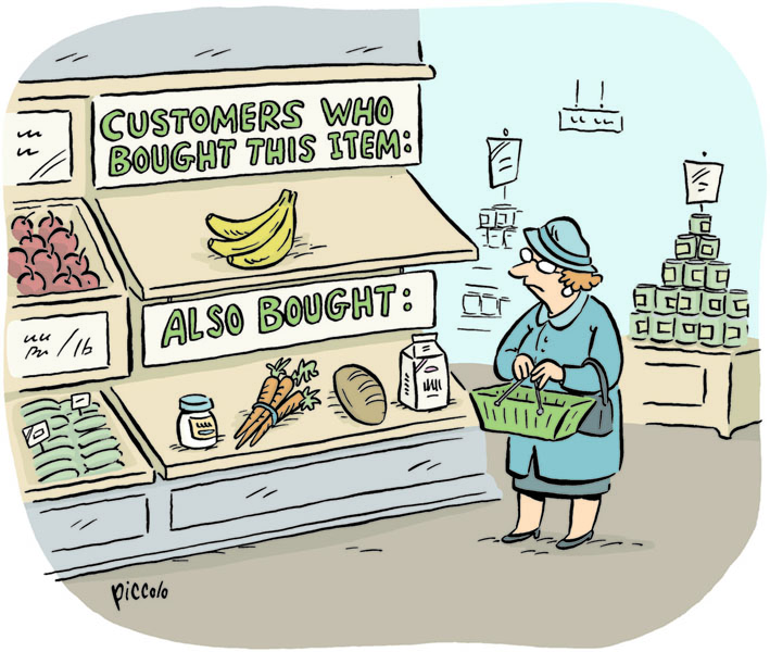
Association Rules
Association rules are usually used in the analysis of product correlations (Market Basket Analysis) and look like this “if there is milk in a customer’s check, then in 80% of cases there will be bread”. That is, if we see that the client has already put the milk in the basket, it's time to remind you of the bread.
This is not the same as the analysis of purchases separated in time, but if we take the whole story as one big basket, we can fully apply this principle here. This can be justified when we, for example, sell expensive one-off goods (credit, flight).
RBM (restricted Bolzman Machines)
Limited Boltzmann machines are a relatively old approach based on stochastic recurrent neural networks. It is a model with latent variables and in this is similar to the SVD decomposition. It also looks for the most compact description of user preferences, which is encoded using latent variables. The method was not designed to find recommendations, but it has been used successfully in top solutions of the Netflix Prize and is still used in some tasks.
Autoencoders (autoencoders)
The basis is still the same principle of spectral decomposition, therefore such networks are also called denoising auto-encoders. The network first collapses the user data known to it into a compact representation, trying to leave only meaningful information, and then restores the data in its original dimension. The result is a certain noise-averaged pattern, which can be used to estimate interest in any product.
DSSM (deep sematic similiarity models)
One of the new approaches. All the same principle, but in the role of latent variables here are internal tensor descriptions of input data (embeddings). Initially, the model was created to match the request with documents (as well as content-based recommendations), but it is easily transformed into the task of matching users and products.
The variety of deep network architectures is limitless, so Deep Learning provides a really wide field for experiments in the field of recommender systems.
In practice, only one approach is rarely used. As a rule, several algorithms are combined into one in order to achieve the maximum effect.
The two main advantages of combining models are an increase in accuracy and the possibility of more flexible tuning to different groups of clients. Disadvantages - less interpretability and greater complexity of implementation and support.
Several merging strategies:
For example, content-based recommender is used, and the result of collaborative filtering is used as one of the features.
Feature Weighted (Linear) Stacking:
Weights are trained on a sample. As a rule, logistic regression is used for this.
Stacking in general:

The Netflix Prize is a competition held in 2009 where it was necessary to predict the assessment of users of the Netflix film library. Not a bad prize of $ 1 million caused a stir and attracted a large number of participants, including quite famous people in the AI.
This was a task with explicit ratings, ratings were set on a scale from 1 to 5, and the accuracy of the forecast was estimated by RMSE. Most of the first places were taken by large classifier ensembles.
The winning ensemble used models of the following classes:
As a meta-algorithm that combined estimates of local algorithms, the traditional gradient boosting was used.
Setting the task of generating recommendations is very simple - we create a matrix of preferences with known user ratings, if it turns out, we supplement these estimates with information on the customer and product, and try to fill in the unknown values.
Despite the simplicity of the statement, there are hundreds of articles that describe fundamentally new methods of its solution. Firstly, this is due to the increasing amount of data collected that can be used in the model and the increasing role of implicit ratings. Secondly, with the development of deep learning and the emergence of new neural network architectures. All this multiplies the complexity of the models.
But in general, all this diversity boils down to a very small set of approaches, which I tried to describe in this article.
Collaborative filtering (Item-based option)
The Item-based approach is a natural alternative to the classic User-based approach, described in the first part, and almost repeats it, except for one thing - it applies to the transposed preference matrix. Those. looking for close products, not users.
Let me remind you, user-based CF (user-based CF) searches for each client a group of the most similar to it (in terms of previous purchases) customers and averages their preferences. These average preferences serve as recommendations for the user. In the case of commodity-based collaborative filtering (item-based CF), the nearest neighbors are searched for on a variety of products — columns of a preference matrix. And the averaging occurs exactly according to them.
Indeed, if the products are meaningfully similar, then most likely they either at the same time like them or at the same time dislike them. Therefore, when we see that the two products have a strong correlation between the estimates, this may indicate that these are equivalent products.
Advantages of Item-based over User-based:
- When there are many users (almost always), the task of finding the nearest neighbor becomes poorly computable. For example, for 1 million users you need to calculate and store
 ~ 500 billion distances. If the distance is encoded in 8 bytes, this is 4TB for the distance matrix alone. If we make Item-based, then the computational complexity decreases with
 before
  and the distance matrix has a dimension no longer (1 million per 1 million) but, for example, (100 per 100) in terms of the number of goods.
 - Assessment of the proximity of products is much more accurate than the assessment of the proximity of users. This is a direct consequence of the fact that there are usually many more users than goods, and therefore the standard error in calculating the correlation of goods there is significantly less. We just have more information to make a conclusion.
- In the user-based version of the description of users, as a rule, they are very sparse (there are a lot of goods, few evaluations). On the one hand, this helps to optimize the calculation - we multiply only those elements where there is an intersection. But on the other hand - how many neighbors do not take, the list of goods that you can recommend in the end is very small.
- User preferences may change over time, but the description of the goods is much more stable.
The rest of the algorithm almost completely repeats the User-based version: the same cosine distance as the main measure of proximity, the same need for data normalization. The number of neighboring goods N is usually chosen in the region of 20.
Due to the fact that the correlation of products is considered on a larger number of observations, it is not so critical to recalculate it after each new assessment and this can be done periodically in batche mode.
Several possible improvements to the algorithm:
- An interesting modification is to consider the “similarity” of products not as a typical cosine distance, but comparing their content (content-based similarity). If at the same time user preferences are not taken into account in any way, such filtering is no longer “collaborative”. At the same time, the second part of the algorithm — obtaining average estimates — does not change at all.
- Another possible modification is to weigh users when calculating item similarity. For example, the more the user made assessments, the more weight he had when comparing two products.
- Instead of simply averaging the estimates for neighboring products, weights can be selected, making linear regression.
When using the item-based approach, recommendations tend to be more conservative. Indeed, the spread of recommendations is less and therefore less likely to show non-standard products.
If in the matrix of preferences we use the review of the description of the product as a rating, then the recommended products will most likely be analogues - products that are often viewed together. If the ratings in the matrix of preferences, we expect on the basis of purchases, then most likely the recommended products will be accessories - products that are often bought together.
System quality assessment
Testing a recommender system is a difficult process and always causing many questions, mainly due to the ambiguity of the very concept of “quality”.
In general, in problems of machine learning there are two main approaches to testing:
- offline testing of the model on historical data using retro tests,
- testing the finished model using A / B testing (we run several options, see which one gives the best result).
Both of these approaches are actively used in the development of recommender systems. Let's start with offline testing.
The main constraint that we face is that we can assess the accuracy of the forecast only on those products that the user has already rated.
The standard approach is cross-validation with the leave-one-out and leave-p-out methods. Multiple repetition of the test with averaging results provides a more stable assessment of quality.
- leave-one-out - the model is trained on all objects, evaluated by the user, except one, and is tested on this one object. This is done for all n objects, and an average is calculated among the obtained n quality estimates.
- Leave-p-out is the same, but at each step p points are excluded.
All quality metrics can be divided into three categories:
- Prediction Accuracy - estimate the accuracy of the predicted rating,
- Decision support - assess the relevance of the recommendations,
- Rank Accuracy Metrics - evaluate the quality of ranking recommendations issued.
Unfortunately, there is no single recommended metric for all occasions, and everyone who is involved in testing a recommender system selects it to fit its goals.
When ratings are rated on a continuous scale (0-10), as a rule, Prediction Accuracy class metrics are sufficient.
| Title | Formula | Description |
|---|---|---|
| MAE (Mean Absolute Error) |  | Mean absolute deviation |
| MSE (Mean Squared Error) |  | RMS error |
| RMSE (Root Mean Squared Error) |  | Root mean square error |
| Title | Formula | Description |
|---|---|---|
| Precision |  | Share recommendations liked by the user |
| Recall |  | Share of user interesting products, which is shown |
| F1-Measure |  | Mean harmonic metrics from Precision and Recall. It is useful when it is impossible to say in advance which of the metrics is more important. |
| ROC AUC | How high is the concentration of interesting products at the beginning of the list of recommendations | |
| Precision @ N | Precision metric counted on Top-N records | |
| Recall @ N | Recall metric counted on Top-N records | |
| Averagep | The average value of precision on the entire list of recommendations |
| Title | Formula | Description |
|---|---|---|
| Mean Reciprocal Rank |  | At what position of the list of recommendations does the user find the first one useful |
| Spearman correlation | | Correlation (Spearman) of real and predictable ranks of recommendations |
| nDCG |  | Informativeness of issue with regard to ranking recommendations |
| Fraction of Concordance Pairs |  | How high is the concentration of interesting products at the beginning of the list of recommendations |
- inform the user about an interesting product,
- to induce him to make a purchase (by mailing, making a personal offer, etc.).
As in any model aimed at motivating the user to action, only incremental increment of the target action should be evaluated. Ie, for example, when calculating purchases on the recommendation, we need to exclude those that the user himself would have done without our model. If this is not done, the effect of the introduction of the model will be greatly overestimated.
Lift is an indicator of how many times the accuracy of a model exceeds a certain baseline algorithm. In our case, the baseline algorithm may simply be the lack of recommendations. This metric well captures the share of incremental purchases and this allows you to effectively compare different models.
Testing with the user
User behavior is a thing that is poorly formalized and not a single metric will fully describe the thought processes in his head when choosing a product. Many factors affect the decision. Follow the link with the recommended product is not yet its high score or even interest. Partially understand the logic of the client helps online testing. Below are a couple of scenarios for such testing.
The first and most obvious scenario is the analysis of site events. We look at what the user does on the site, whether he pays attention to our recommendations, whether he follows them, which features of the system are in demand, which are not, which products are better recommended, and which are worse. To understand which of the algorithms as a whole works better or just try a new promising idea, we do A / B testing and collect the result.
The second scenario is receiving feedback from users in the form of polls and polls. As a rule, these are general questions for understanding how customers use the service — which is more important: relevance or diversity, is it possible to show duplicate products, or is it too annoying. The advantage of the script is that it gives a direct answer to all these questions.
Such testing is difficult, but for large reference services, it is simply necessary. Questions may be more complex, for example, “which of the lists seems to be more relevant to you,” “how much the sheet looks solid,” “whether you will watch this film / read a book”.
Implicit ratings and unary data
At the beginning of its development, recommender systems were used in services where the user explicitly assesses the product by rating him — this is Amazon, Netflix, and other Internet commerce sites. However, with the growing popularity of recommender systems, the need has arisen to apply them even where there are no ratings - these can be banks, car repair shops, shawarma stalls, and any other services where, for some reason, it is impossible to establish an assessment system. In these cases, the user's interests can be calculated only by indirect signs - certain actions with the product, for example, viewing the description on the site, adding the product to the basket, etc., tell about user preferences. It uses the principle of "bought - it means love!". Such an implicit rating system is called Implicit Ratings.
Implicit ratings obviously work worse than explicit ones, because they make an order of magnitude more noise. After all, the user could buy goods as a gift to his wife or go to the page with a description of the goods, only to leave a comment there in the style of “what is it nonetheless” or satisfy his natural curiosity.
If, in the case of explicit ratings, we have the right to expect that at least one negative assessment no-no and even put it, then we will not take a negative assessment from nowhere. If the user did not buy the book Fifty Shades of Gray, he could do it for two reasons:
- she is really not interested in him (this is a negative case),
- She is interested in him, but he just does not know about her (this is a missed positive case).
But we have no data to distinguish the first case from the second. This is bad, because when teaching a model, we have to back it up on positive cases and fine it on negative ones, and we will almost always fine it, and as a result, the model will be biased.
The second case is an opportunity to leave only positive marks. A vivid example is the Like button in social networks. The rating here is set down explicitly, but just like in the previous example, we have no negative examples - we know which channels the user likes, but we don’t know which channels do not like.
In both examples, the task becomes a Unary Class Classification task .
The most obvious solution is to follow a simple path and consider the lack of an assessment to be a negative assessment. In some cases this is more justified, in some less so. For example, if we know that the user has most likely seen the product (for example, we showed it to him in the list of products, and he switched to the product that goes after him), then the lack of a transition can really indicate a lack of interest.
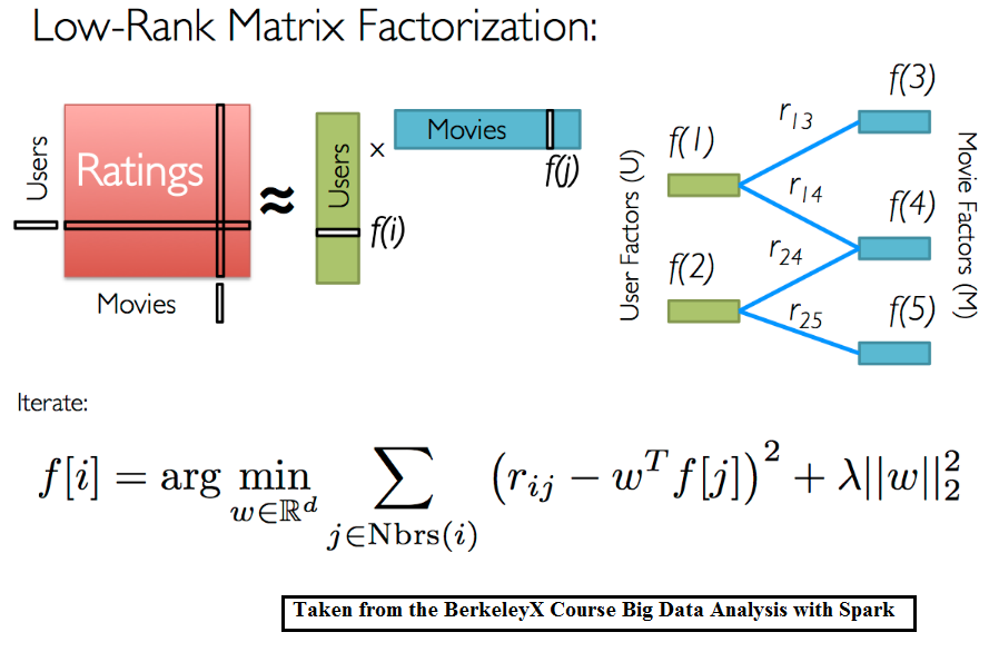
Algorithms of factorization
It would be great to describe the interests of the user in more "large strokes". Not in the format of "he loves films X, Y and Z", but in the format of "he loves modern Russian comedies." Besides the fact that it will increase the generalizability of the model, it will also solve the problem of large data dimension - after all, the interests will be described not by the goods vector, but by a significantly smaller preference vector.
Such approaches are also called spectral decomposition or high-frequency filtering (since we remove the noise and leave the useful signal). In algebra, there are many different decompositions of matrices, and one of the most commonly used is called SVD decomposition (singular value decomposition).
The SVD method was used in the late 80s to select pages that were similar in meaning, but not in content, and then began to be used in recommendations. The method is based on the decomposition of the initial rating matrix ® into a product of 3 matrices:
where matrix sizes and r - the rank of the decomposition - a parameter characterizing the degree of detail of the decomposition.
Applying this decomposition to our matrix of preferences, we get two matrixes of factors (abbreviated descriptions):
U is a compact description of user preferences,
S is a compact description of product characteristics.
It is important that with this approach we do not know which particular characteristics correspond to the factors in the reduced descriptions; for us they are encoded with some numbers. Therefore, SVD is an uninterpreted model.
In order to obtain an approximation of the matrix of preferences, it is sufficient to multiply the matrix of factors. By doing this, we get a rating for all customer-product pairs.
A common family of such algorithms is called NMF (non-negative matrix factorization). As a rule, the calculation of such expansions is very laborious, therefore, in practice, they often resort to their approximate iterative variants.
ALS (alternating least squares) is a popular iterative algorithm for decomposing a matrix of preferences into a product of 2 matrices: user factors (U) and product factors (I). Works on the principle of minimizing the root-mean-square error on the affixed ratings. Optimization takes place alternately, first by user factors, then by product factors. Also, to avoid retraining, the regularization coefficients are added to the root-mean-square error.
If we supplement the matrix of preferences with a new dimension containing information about the user or product, then we will be able to lay out not the matrix of preferences, but the tensor. Thus, we will use more available information and possibly get a more accurate model.
Other approaches
Association Rules
Association rules are usually used in the analysis of product correlations (Market Basket Analysis) and look like this “if there is milk in a customer’s check, then in 80% of cases there will be bread”. That is, if we see that the client has already put the milk in the basket, it's time to remind you of the bread.
This is not the same as the analysis of purchases separated in time, but if we take the whole story as one big basket, we can fully apply this principle here. This can be justified when we, for example, sell expensive one-off goods (credit, flight).
RBM (restricted Bolzman Machines)
Limited Boltzmann machines are a relatively old approach based on stochastic recurrent neural networks. It is a model with latent variables and in this is similar to the SVD decomposition. It also looks for the most compact description of user preferences, which is encoded using latent variables. The method was not designed to find recommendations, but it has been used successfully in top solutions of the Netflix Prize and is still used in some tasks.
Autoencoders (autoencoders)
The basis is still the same principle of spectral decomposition, therefore such networks are also called denoising auto-encoders. The network first collapses the user data known to it into a compact representation, trying to leave only meaningful information, and then restores the data in its original dimension. The result is a certain noise-averaged pattern, which can be used to estimate interest in any product.
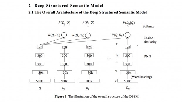
DSSM (deep sematic similiarity models)
One of the new approaches. All the same principle, but in the role of latent variables here are internal tensor descriptions of input data (embeddings). Initially, the model was created to match the request with documents (as well as content-based recommendations), but it is easily transformed into the task of matching users and products.
The variety of deep network architectures is limitless, so Deep Learning provides a really wide field for experiments in the field of recommender systems.
Hybrid solutions
In practice, only one approach is rarely used. As a rule, several algorithms are combined into one in order to achieve the maximum effect.
The two main advantages of combining models are an increase in accuracy and the possibility of more flexible tuning to different groups of clients. Disadvantages - less interpretability and greater complexity of implementation and support.
Several merging strategies:
- Weighting - calculate the weighted average forecast by several estimates.
- Stacking - the predictions of individual models are the inputs of another (meta) classifier, which is trained to correctly weigh the intermediate estimates,
- Switching - for different products / users to use different algorithms,
- Mixing - recommendations are calculated for different algorithms, and then simply combined into one list.
For example, content-based recommender is used, and the result of collaborative filtering is used as one of the features.
Feature Weighted (Linear) Stacking:

Weights
are trained on a sample. As a rule, logistic regression is used for this. Stacking in general:

Netflix Solution Brief
The Netflix Prize is a competition held in 2009 where it was necessary to predict the assessment of users of the Netflix film library. Not a bad prize of $ 1 million caused a stir and attracted a large number of participants, including quite famous people in the AI.
This was a task with explicit ratings, ratings were set on a scale from 1 to 5, and the accuracy of the forecast was estimated by RMSE. Most of the first places were taken by large classifier ensembles.
The winning ensemble used models of the following classes:
- basic model - regression model based on averages
- collaborative filtering - collaborative filtering
- RBM - Boltzmann Limited Machines
- random forests - predictive model
As a meta-algorithm that combined estimates of local algorithms, the traditional gradient boosting was used.
Summary
Setting the task of generating recommendations is very simple - we create a matrix of preferences with known user ratings, if it turns out, we supplement these estimates with information on the customer and product, and try to fill in the unknown values.
Despite the simplicity of the statement, there are hundreds of articles that describe fundamentally new methods of its solution. Firstly, this is due to the increasing amount of data collected that can be used in the model and the increasing role of implicit ratings. Secondly, with the development of deep learning and the emergence of new neural network architectures. All this multiplies the complexity of the models.
But in general, all this diversity boils down to a very small set of approaches, which I tried to describe in this article.
I remind about our vacancies.