Motion planning: graph of visibility, roadmaps
Good day to all. In this article I would like to talk about a couple of algorithms related to computational geometry, which are currently widely used in game development. If you have at least once programmed a game in which there is a character (s) moving around a location, you had to solve the problem of finding the path. I want to talk about one of the approaches to solving this problem.
Formulation of the problem
Let a set of disjoint polygons P - polygonal obstacles be given. Let there be an agent moving in the same plane — it is represented by a dot. Let the starting point s and the ending point f be given. We need to build the shortest route from point s to point f, while we assume that the agent can be on the border of the obstacle, but not inside it.
Decision
Optimal way
It can be proved that the optimal path is a piecewise linear broken line whose vertices coincide with the vertices of the obstacles.
Evidence
Part 1. The optimal path is a piecewise linear broken line.
Suppose that the shortest path T is not a piecewise linear broken line. In this case, on the path T there exists a point p that does not belong to any straight segment from T (Figure 1). This means that there is an ε-neighborhood of the point p (Figure 2) at which no obstacle falls. In this case, the subpath T ε that is inside the ε-neighborhood can be shortened along the chord connecting the points of intersection of the boundary of the ε-neighborhood with the path T. Since part of the path can be reduced, then the whole path can be reduced, and therefore the original the assumption is incorrect. The path T is a piecewise linear broken line.
Part 2. The vertices of the path coincide with the vertices of the obstacles.
Now suppose that the vertices of the path T do not coincide with the vertices of the obstacle polygons. Consider the vertex v of the path T. The vertex cannot lie inside the free space, because otherwise, using a similar approach, we would find a shorter path along the chord in the ε-neighborhood of the vertex v (Figure 4). Hence, the vertex v must lie on the boundaries of obstacles (at their vertices or on the edges). But the vertex cannot lie on the edges either, since (again we consider the ε-neighborhood), we can cut along the chord (Figure 5).
The above means that the vertices of the piecewise linear path T must be located at the vertices of the obstacles-polygons.
Suppose that the shortest path T is not a piecewise linear broken line. In this case, on the path T there exists a point p that does not belong to any straight segment from T (Figure 1). This means that there is an ε-neighborhood of the point p (Figure 2) at which no obstacle falls. In this case, the subpath T ε that is inside the ε-neighborhood can be shortened along the chord connecting the points of intersection of the boundary of the ε-neighborhood with the path T. Since part of the path can be reduced, then the whole path can be reduced, and therefore the original the assumption is incorrect. The path T is a piecewise linear broken line.
 |  |  |
Figure 1. Point p on path T | Figure 2. ε-neighborhood of p | Figure 3. The shortest path chord |
Part 2. The vertices of the path coincide with the vertices of the obstacles.
Now suppose that the vertices of the path T do not coincide with the vertices of the obstacle polygons. Consider the vertex v of the path T. The vertex cannot lie inside the free space, because otherwise, using a similar approach, we would find a shorter path along the chord in the ε-neighborhood of the vertex v (Figure 4). Hence, the vertex v must lie on the boundaries of obstacles (at their vertices or on the edges). But the vertex cannot lie on the edges either, since (again we consider the ε-neighborhood), we can cut along the chord (Figure 5).
 |  |
Figure 4. ε-neighborhood of the top of the path lying in free space | Figure 5. ε-neighborhood of the top of the path lying on the edge |
The above means that the vertices of the piecewise linear path T must be located at the vertices of the obstacles-polygons.
Visibility graph
We will call two points mutually visible if the segment connecting them does not contain internal points of obstacles-polygons.
To construct the shortest path, a visibility graph is used. The vertices of the graph are the vertices of the obstacles-polygons. Only mutually visible vertices of the graph are connected by edges.

Figure 6. An example of a visibility graph.
Suppose we have built a visibility graph VG. Add the vertices s and f to the graph VG, as well as the edges connecting them with all the vertices visible from them. We get the extended graph VG + . All that remains for us is to find the shortest path from the vertex s to the vertex f in the graph VG + . This can be done by applying Dijkstra's algorithm . I will not talk about it in detail, since there are a huge number of articles on the Internet, including on the Habr . It remains only to solve the problem of constructing a visibility graph.
Building a visibility graph: a naive algorithm
We will sort through all pairs of vertices in the graph VG + and for each of them we will check to see if the segment connecting the vertices of the obstacle edge intersects. It is easy to see that the complexity of such an algorithm is O (n 3 ), since we have n 2 pairs of vertices and O (n) edges.
Building a visibility graph in O (n 2 log (n))
Let's try to build a visibility graph a little faster. For each vertex, we find all the vertices visible from it using the planar sweeping method. We need to solve the following problem: on the plane are given many segments (obstacle edges) and a point p. Find all the ends of the segments visible from the point p. We will sweep the plane with a rotating beam with a beginning at point p (Figure 7). The status of the sweeping line will be the segments that intersect it, ordered by increasing distance from point p to the intersection point. The points of events will be the ends of the segments.

Figure 7. Sweeping a plane with a rotating beam
The vertices ordered by the angle relative to the axis passing through point p will be stored in the event queue. Initialization of the status will take O (nlog (n)) time, initialization of the event queue will also take O (nlog (n)) time. The total operating time of the sweeping algorithm is O (nlog (n)), thus, applying the algorithm for each vertex of the graph, we obtain a visibility graph over time of the order of O (n 2 log (n)).
More formally. Let the number of edges of the set of disjoint polygons-obstacle be n. In spoilers, I will cite code in a pseudo-language that is as similar to Java as possible.
Building a visibility graph
public final G buildVisibilityGraph(final Set segments) {
  /* Инициализация графа. Добавление всех концов отрезков в качестве вершин графа. Множество рёбер - пустое.  */
  final G visibilityGraph = new G(getVertices(segments));
  /* Для каждой вершины графа */
  for (final Vertex v : visibilityGraph.getVertices()) {
    /* Получение всех видимых из неё вершин */
    final Set visibleVertices = getVisibleVertices(v, segments);
    /* Создание рёбер для всех видимых вершин */
    for (final Vertex w : visibleVertices)
      visibilityGraph.addEdge(v, w);
  }
  return visibilityGraph;
}
The buildVisibilityGraph function accepts a lot of segments - edges of obstacle polygons - as an input and returns the constructed visibility graph. Explanations here, it seems to me, are not required. Consider the pseudocode of the getVisibleVertices function.
Getting a list of all visible vertices
public final Set getVisibleVertices(final Vertex v, final Set segments) {
  /* Сортировка всех вершин (концов отрезков) по углу, образуемому отрезком pw (где w - конец отрезка) с вертикальной полуосью, проходящей через вершину v */
  final SortedSet sortedVertices = sortSegmentsVertices(v, segments);
  /* Пусть I - вертикальная полуось, проходящая через v. Найдём все отрезки, пересекающие эту ось и занесем их в в сбалансированное дерево поиска в порядке удаленности точки пересечения с полуосью */
  final BST intersectedSegments = new BST(v, segments);
  /* Изначально нет видимых вершин */
  final Set visibleVertices = new HashSet();
  /* Заметание плоскости по углу */
  for (final Vertex w : sortedVertices) {
    if (isVertexVisible(v, w, intersectedSegments))
      visibleVertices.add(w);
    /* Добавление в список пересечений всех рёбер, инцидентных вершине w и лежащих справа от заметающей прямой (луча vw), иными словами, начинающихся в вершине w */
    intersectedSegments.add(getIncidentSegments(v, w, Position.RightOf));
    /* Удаление из списка пересечений всех рёбер, инцидентных вершине w и лежащих слева от заметающей прямой (луча vw), иными словами, заканчивающихся в вершине w */
    intersecedSegments.remove(getIncidentSegments(v, w, Position.LeftOf));
  }
  return visibleVertices;
}
So, first of all, the vertices w ∈ W are sorted by the angle between the ray vw and the vertical half-axis passing through v. This sorting is done in O (nlog (n)), for example, merge sorting. Then, the set of visible vertices is initialized (by default, such a set is empty). Next begins sweeping the plane. In the order of sorting the vertices for each of them, a check is made: is the vertex w visible from the vertex v. Since this check means there are intersections that are stored in a balanced tree, it can be done in O (log (n)). If a vertex is visible, add it to the list of visible vertices. And finally, regardless of the visibility of the peak, it is necessary to change the status of the sweeping line. To do this, for the current vertex w, it is necessary to remove all edges (segments) from the list of current intersections,
Consider Figures 8-10:
Figures 8-10


Figure 8. Step 1. Updating the status of the sweeping line.
Figure 9. Step 2. Updating the status of the sweeping line.
Figure 10. Step 3. Updating the status of the sweeping line.
So, at the first step (ray vw 1 ), two segments w 1 w 5 and w 1 w 2 are added to the tree , since they lie to the right of ray vw 1 . The status of the swept line is marked in orange.
At the second step (the second vertex in the list is the vertex w 3 ), two more edges are added to the status: w 3 w 2 and w 3 w 4 . Now 4 ribs are in status. Finally, in the third step (vertex w 2 ), 2 edges are removed from the status: w 3 w 2 and w 1 w 2 .
Ultimately, you should look at the vertex visibility check function.
Verification Visibility Function
public final boolean isVisible(final Vertex v, final Vertex w, final BST intersections) {
  final Segment currentSegment = new Segment(v, w);
  /* Отрезок vw всегда пересекается с отрезками, инцидентными вершине w, поэтому исключаем их */
  if (intersects(currentSegment, w.getSegments())
    return false;
  /* Предыдущая вершина (по углу) лежит на отрезка vw. */
  if (currentSegment.contains(w.getPreviousVertex())) {
    /* Предыдущая вершина невидима, отрезок продолжается, никаких изменений */
    if (!v.getPreviousVertex().isVisible())
      return false;
    return !intersections.hasIntersectionsWith(new Segment(w.getPrevious(), w));
  }
  /* Проверка на пересечение луча с самым левого листом (самое близкое пересечение луча vw с отрезком из статуса) */
  return intersections.intersectWithLeftMost(currentSegment);
}
This function just needs to return true if the vertex w is visible from the vertex v and false otherwise. To do this, it is enough just to compare the length of the segment vw and the distance from the point v to the intersection with the nearest segment stored in the tree (the leftmost sheet). But here there are several boundary cases:
- Ray vw crosses edges incident to vertices v or w
- The ray coincides with the edge on which the other vertices are.
Thus, the visibility check function works in the worst case for O (log (n)), since it uses a search in a balanced tree. The remaining operations are performed in constant time.
Road maps
Another route planning method is using roadmaps. Sounds like a truism, right? In the framework of this article, I will briefly talk about its essence (because the article is already quite lengthy), if anyone is interested, maybe I will write another publication later. So.
Let's build a rectangle containing all the obstacle polygons inside it (Figure 11). Consider the set of segments - edges of obstacles and construct a trapezoidal map for it (Figure 12), and then remove from the resulting map all trapezoids lying inside the obstacles (Figure 13). It takes O (nlog (n)) time to build a map, where n is the total number of obstacle vertices. In order to decide whether to remove the trapezoid T, it suffices to take the edge top (T) and check whether an obstacle lies at the top or bottom of it, the boundary of which contains this edge. Thus, it takes O (n) time to remove all the extra trapezoids.
If the start and end points are inside the same trapezoid, then you can go from the first point to the second in a straight line. If these points lie in different trapezoid, then the path will cross several trapezoid, and, probably, in some of them we will have to make turns.
Let's build a road map - graph G. The vertices of G will be the midpoints of the vertical lines drawn through the tops of the obstacles and the midpoints of the trapezoid. Two vertices of the graph G are connected by an edge if and only if one of them is the middle of some trapezoid and the other lies on the vertical edge of this trapezoid. Graph G can be constructed from a trapezoidal map in time O (n). Note that the graph G is a flat graph.
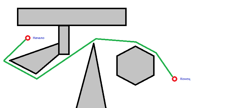
In order to find the path from point s to point f, we first determine which trapezoid contains s and f. If they got inside one trapezoid, then the shortest path is a straight line. Otherwise, we move in a straight line from point s to the middle of the trapezoid containing it, then move along the edges of the graph to the middle of the trapezoid containing f (you can use the breadth-first search), and finally move to f in a straight line from the middle of the trapezoid (figure 14). Since the trapezoidal map contains the number of trapezoids linear in n, and the number of segments of vertical lines drawn through the vertices of the obstacles is also linear in n, the graph G has O (n) vertices, and since it is planar, the number of edges is also O ( n). Therefore, a breadth-first search on G can be done in time O (n). Since time O (log (n)) is required to localize a point in a trapezoidal map, time O (n) is required to construct a path from point s to point f. But the paths built using roadmaps will not be optimal.
 |  |  |
Figure 11. Building an enclosing rectangle | Figure 12. Trapezoidal map | Figure 13. The reduced trapezoidal map |

Figure 14. The constructed road map
Subtasks
Convex hull construction
In general, a scene is a collection of arbitrary objects. For each of them, a convex hull can be constructed (well, or a bounding volume, if great accuracy is not needed or all objects look like rectangles). In order to be able to use the visibility graph for arbitrary geometry, it is necessary to map it to many polygons. The simplest way is to build a convex hull. There are several different algorithms for its construction and this is a topic for a separate article, I will only mention them here:
- The naive algorithm. Works for O (n 4 ). For each “not extreme” (that is, such a point of the set through which you can draw a straight line with respect to which the whole set will lie on one side), the following test is performed. If it belongs to at least one triangle obtained from the points of the set, then it is a point of the convex hull. In a set of N points, there are N 3 triangles. Therefore, for each of the N points, you need to perform N 3 checks.
- A slightly less naive algorithm. O (n 3 ). A complete graph is constructed with many nodes — points of the original set. For each edge (of which N 2 ) the remaining N-2 points are checked. Do they all lie on one side of a given rib. If so, then the edge belongs to the convex hull.
- Jarvis Algorithm. Works for O (n 2 ). Imagine a lot of points on a plane. Choose the leftmost among them (this can always be done (if there are several, then any among the left), it is obviously the point of the convex hull), and then “wrap” the set as a gift. Among all other points, we choose one that has the smallest polar angle (by analogy with the construction of a visibility graph, we spot it with a ray)
- Graham Algorithm. Works for O (nlog (n)). I will not provide a description (as you know, the faster the algorithm, the more scribble) - google
Line intersection
Finally, the last task that needs to be solved within the framework of constructing a visibility graph is to check two segments for intersections. This is a very good topic for a separate article, since there is quite a lot to write on this issue. I will only give one of the methods of solving the problem that I liked: here it is .
Conclusion
I hope someone thought the article was interesting, and maybe even useful. In the near future I plan to publish another article, and then it will be seen - we will arrange a survey on whether to continue.
Instead of a thousand words
References
- Lecture courses in linear algebra, higher mathematics, discrete mathematics, theory of algorithms and computational geometry at the Department of Applied Mathematics, St. Petersburg State Pedagogical University
- M. de Berg, O. Cheong, M. Kreveld, M. Overmars Computational Geometry, 2008
- JE Goodman, J. O'Rourke Discrete and computational geometry, 2004
- Venta library implementation in Java