CFD 3D: a simple water simulator
 |  |
Introduction
CFD (Computational fluid dynamics) - computational fluid dynamics.
It is used to simulate different processes in liquids, as well as different types of liquids (for example, honey, oil - these are all liquids).
In this post, a 2D simulator of ordinary water with an open surface and obstacles is considered (for the 3D version, everything is similar + the source is available ).
The surface of the water is the boundary separating the water from the air. This allows you to simulate waves, droplets, etc.
I decided to write my simulator for several reasons. One of them is the lack of properly written sources on this topic on the Internet. All that I found was either on Fortran, or only 2d, or it was written very hard to understand.
So, the main features of the simulator:
- real-time mode
- simple and clear calculation scheme + explicit, implicit
- open source
- there are 2d and 3d
- built-in simple opengl render
- xml scene description
In terms of calculations, I started from the Navier-Stokes equations (as well as from the sources found on the Internet).
This is a system of partial differential equations describing the motion of a viscous incompressible fluid. The word incompressible here is more like a tick, since all liquids are, by definition, incompressible. Viscosity means friction between individual particles; it prevents them from scattering in different directions, as in the case of gas, when it fills the entire volume allocated to it. Liquid particles try to stick together as much as possible.
In my simulator I used a slightly modified set of equations, more on that below ...
Hydrodynamic equations
So, here are the basic Navier-Stokes equations in the general (vector) form:
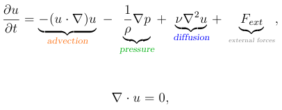
Here:
- u is the traditional designation of the velocity field (in 2D - the velocity consists of 2 components in x and in y directions - they are denoted by u and v, respectively)
- p is the pressure
- t is time
- rho symbol - fluid density
- symbol nu - kinematic viscosity coefficient
- Fext - any external forces acting on a liquid, for example gravity (g)
The first of the equations is the equation of motion, the second is the continuity equation.
The equation of motion looks similar to the Newton equation ma = F, where for us on the right - the sum of the forces acting on the liquid is pressure, diffusion, gravity ...
For the 2D version, the equations take this form (here they are already presented in a dimensionless form):
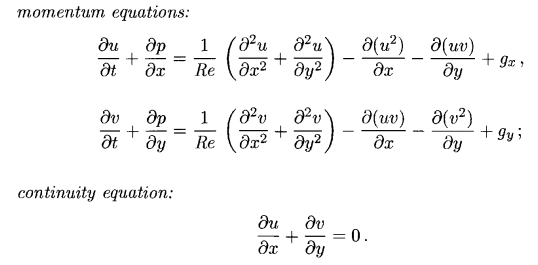
The equation of motion is now presented 2 equations - for 2x velocity components - u and v.
Regarding the new coefficient, Re is the Reynolds number (it turned out when we switched to dimensionless variables), which immediately replaces the 2 previous coefficients - coefficient. density and viscosity. It depends on what the water will look like - like honey or ordinary water. The more Re, the more similar the liquid is to ordinary water.
In parentheses, this is our expression defining the viscous behavior of a liquid (or diffusion). The remaining terms on the right side (except for gravity) are convection. In the left part - speed and pressure.
Further, I simplified these equations a little:

As you can see, convection has disappeared, which slightly worsens the behavior of the liquid, but overall it looks quite normal visually. Lack of convection gives several advantages at once - non-linearity disappears, stability improves and time step can be done more, convection usually a very expensive term in terms of the number of necessary calculations, moreover, in order to correctly discretize convection, special schemes are used - which looks rather cumbersome.
When solving equations, we use a special scheme called Splitting. I would like to dwell on this in more detail, but this is more for a separate post. The topic is quite large. This is very well described in the book
Bridson R. Fluid Simulation for Computer Graphics.pdf in the section Overview of numerical simulation.
And here Numerical simulation in fluid dynamics Griebel M Dornseifer T Neunhoeffer T SIAM 1998
Here is a split equation solution scheme:
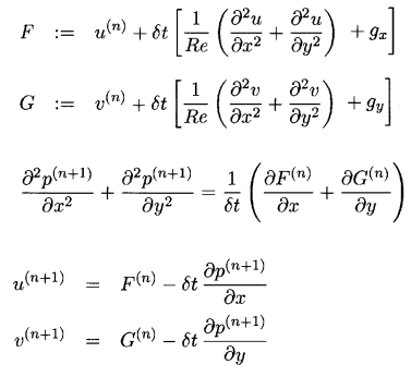
For the time step, the Euler method is used, also at the first step we lower the pressure and obtain an intermediate calculation of the velocities F and G. These velocities, in addition to not taking pressure into account, will also not satisfy the continuity equation. Through tricky manipulations, an equation for calculating the pressure is found, which also solves the problem with the continuity equation. Solving this equation using the already calculated F and G, we find a new pressure P.
Then, at the 3rd step, the velocity is corrected taking into account the calculated pressure.
This completes one complete time step and in the next step everything is repeated anew.
Discretization of Equations
The finite difference method is used to discretize the equations. For the time step, the standard Euler method is used - it schematically looks like this: u (n + 1) = u (n) + dt * f,
where f means the entire part of the equation that does not include the time differential.
In general, the speed value at a new moment in time (u (n + 1)) is found from the value at the previous moment in time (u (n)).
I will not describe discrete analogs of equations in this post. This is very well done in the book Numerical simulation in fluid dynamics (Griebel M Dornseifer T Neunhoeffer T SIAM 1998).
To solve discrete equations, it is not the matrix method of solution that is used, but the iterative Gauss-Seidel method. It does not require preliminary assembly of matrices and generally does not require any intermediate arrays, it allows you to easily modify the calculation scheme, an approximate solution is already after 1 iteration - which greatly accelerates the entire simulation.
In this post, we will consider the 2D case, the main emphasis will be on explaining the boundary conditions, since they cause the greatest difficulty in solving equations. The entire simulated area is divided into imax points horizontally and jmax vertically. It turns out a grid of imax * jmax cells.
Boundary points are added to them from 4 borders. In total, an array of size (imax + 2) * (jmax + 2) is obtained.
Each cell has its own values of velocities and pressure - it is customary to talk about the vector velocity field and the scalar pressure field on the computational grid.
U - particle velocity in the cell in x
V - particle velocity in the cell in y
P - pressure
It is customary to arrange the calculated variables (U, V, P) in the center of the cells, but in the case of fluid modeling this always causes problems with the solution - it turns out not quite correct and oscillating. Therefore, the CFD uses a staggered grid - it is also called leapfrog.
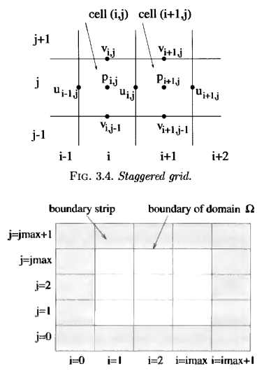
It can be seen from the figure that the velocities are not in the cell itself but on its faces, u - on the right border of the cell, and v - on the upper border.
Boundary conditions on the walls
To calculate by the finite difference method, we need to set the values (u, v, p) at the borders of the computational grid. These are 4 walls - from left to bottom and top right. The boundary conditions can be of no-slip and free-sleep types; there are other types, but these are more specialized conditions, rather than a general plan.
free-sleep - this means that the liquid glides freely along the wall, as if there is no friction and nothing prevents it from moving along it.
In this post we do not consider this type of boundary conditions.
no-slip is a sticking condition - that is, a fluid slows down when it hits a wall.
This means that the fluid velocity coincides with the velocity of the wall (that is, in our case it is zero at a fixed boundary).
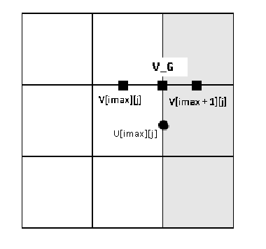
For example, consider only the right boundary: u component of velocity = 0, because it is perpendicular to the wall and water should not penetrate the border.
The v component for the case of a no-slip boundary is also 0, but for our staggered mesh it will be necessary to correct it. For the v component, given that v is not directly on the border, it is necessary to slightly correct the expression.
v on the wall will be equal to the average between the last 2 cells. v_g = (v [imax + 1] [j] + v [imax] [j]) / 2
v_g equal to zero ((v [imax + 1] [j] + v [imax] [j]) / 2 = 0 ) and find from here the value v [imax + 1] [j], which we need to set in the program:
v [imax + 1] [j] = - v [imax] [j];
The same thing needs to be done for the u components on the upper boundary.
4 borders are represented in the array by the following coordinates:
the left wall is
u [0] [j], where j runs over the entire wall
v [0] [j]
Here is what it looks like in the code:
for (j = 0; j <= jmax + 1; j++)
{
  U[0][j] = 0.0;
  V[0][j] = -V[1][j];
}
bottom wall
u [i] [0]
v [i] [0]
for (i = 0; i <= imax + 1; i++)
{
  U[i][0] = -U[i][1];
  V[i][0] = 0.0;
}
Since the right wall of T. Since we have a spaced grid, then on the right wall we have a border for the values of u that passes not along the last column but along the penultimate column - therefore, we set the values for U in the cell to U [imax] [j].
u [imax] [j]
v [imax + 1] [j]
for (j = 0; j <= jmax + 1; j++)
{
  U[imax][j] = 0.0;
  V[imax + 1][j] = -V[imax][j];
}
upper wall
Here, for values of v, the border runs along the penultimate line - jmax - so we set the values for V in the cell - V [i] [jmax]
u [i] [jmax + 1]
v [i] [jmax]
for (i = 0; i <= imax + 1; i++)
{
  U[i][jmax + 1] = -U[i][jmax];
  V[i][jmax] = 0.0;
}
To test the main solver, you can set all boundary values = 0.
We also need to put pressure on the borders. The pressure is set in the center of the cells and not at the edges as the speed. Therefore, it is very simple. The pressure at the borders can be set the same as in neighboring cells. Just copy the values from neighboring cells.
for (j = 1; j <= jmax; j++)
{
  // левая стенка
  P[0][j] = P[1][j];
  // правая стенка
  P[imax + 1][j] = P[imax][j];
}
for (i = 1; i <= imax; i++)
{
  P[i][0] = P[i][1];
  P[i][jmax + 1] = P[i][jmax];
}
Boundary conditions on obstacles
Obstacles are represented by the flag C_B. The boundary conditions for them are set on the same principle as for the external walls. I will give 2 examples of setting the pressure:
if (IsObstacle(i, j))
{
   // если снизу от препятствия - вода - то копируем значение P из нее
          if (IsFluid(i, j - 1))
          {
            P[i][j] = P[i][j - 1];
          }
   // если слева - вода ...
          else if (IsFluid(i - 1, j))
          {
            P[i][j] = P[i - 1][j];
          }
  // .......
}
For an angular cell, we take the average of the values of the water cells surrounding it. For example, take an obstacle, there will be water to the left and above it. Then we consider the pressure in the obstacle cell as follows:
if (IsFluid(i - 1, j) && IsFluid(i, j + 1))
{
  P[i][j] = (P[i][j + 1] + P[i - 1][j]) / 2;
}
Boundary conditions on the surface
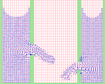
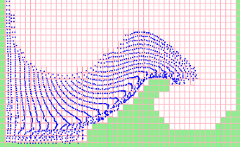
The surface and its motion are modeled using particles. (Sources with boundary conditions on the surface, made as described in this section, are in the simpletestobstacle folder.)
Initially, particles are placed in cells with liquid, 4 pieces per cell (1 near each corner). Next, the particles at each step move using the simple Euler method from classical mechanics. The speeds for movement are taken in each cell as the average for the whole cell (although it is not a problem to use, for example, interpolation).
  x = particles[k].x;
  y = particles[k].y;
// определяем координаты клетки в которой находятся частицы
  i = (int)(x / delx);
  j = (int)(y / dely);
  u = U[i][j];
  v = V[i][j];
  // собственно сам метод Эйлера для движения частиц
  x += delt * u;
  y += delt * v;
At each step, cells with particles are labeled as water. The rest are empty cells; the basic variables (u, v, p) are not calculated in them.
To calculate the main variables, it is necessary to set the boundary conditions on the surface and adjacent cells, just as it was required for the walls. But first you need to determine which cells, of those labeled as water, belong to the surface, and also from which side the air is. For these purposes, 2 arrays are used - FLAG and FLAGSURF. In the first, only cell types are specified - water, air (empty) and obstacles. Here are the corresponding flags (abbreviations B - boundary F - fluid E - empty):
public const int C_B = 0x0000; //препятствие
public const int C_F = 0x0010;//вода
public const int C_E = 0x1000;//пусто
The FLAGSURF array is used to determine surface cells; for the remaining cells, the value there = 0. The flags in this array determine not only the type of cell, but also all combinations of neighboring cells in which it is empty. Flags are made as standard bit masks so that they can be combined.
Each value in FLAGSURF contains 4 bits that correspond to 4 sides (adjacent cells).
If the bit is set to 1 then in the corresponding neighboring cell - empty. If 0 - then there is water.
Bit location: 0000 NSWO 0000 0000 - the letters indicate the 4 sides of N (North North) S (South South) W (West East) and O (West).
The entire list of flags is in the source, so I will give only some examples of values:
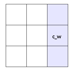
public const int C_W = 0x0200; // 512
in binary form, the value looks like 0000 0010 0000 0000
Here the flag corresponding to the W side is set to 1. This means that to the left of the current cell is empty.
At the same time, the remaining 3 bits are set to 0, which means the remaining neighboring cells are filled with water.
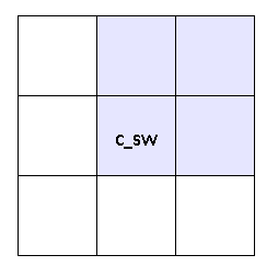
public const int C_SW = 0x0600; // 1536 0000 0110 0000 0000
Here the flag corresponding to the sides W and S is set to 1. It means to the left and bottom of the current cell that it is empty, and the remaining cells that are water.
When determining the types of surface cells and filling in the FLAGSURF array, the corresponding bits are set to 1 this way:
// если слева пусто, то установим соответствующий бит  в 1
if (FLAG[i-1][j] == GG.C_E)
  FLAGSURF[i][j] = FLAGSURF[i][j] | GG.C_W;
The FLAGSURF array is mainly needed only for the convenience of setting boundary conditions on the surface. Since for different types of surface cells different boundary conditions apply. As already mentioned, we need to put down the boundary conditions in the empty cells that are next to the surface cells and also the boundary conditions are needed in the surface cells themselves, since we have a staggered grid and not all surface cells are included in the calculation of uv variables.
The principle of setting values is simple. Because air pressure is 1000 times less than pressure in water - it can be neglected and allowed water to move freely along the surface, without limiting its speed and without changing the direction of movement. Of course, in my scheme surface tension is not taken into account, otherwise everything would have been much more complicated.
We put down the values of the velocities U and V in the surface cells and the empty cells bordering them, without forgetting that we have a staggered grid.
Values for placement are taken from neighboring water cells. It remains only to decide from which neighboring cells all this is taken, because there can be several such cells.

Here is a screen with boundary conditions that need to be put down. Blue squares are water. Black marks are the required boundary conditions. Note that the labels are located partially in the surface cells and partially in the empty cells. This happens because in the solver code we have such conditions (as you can see, UV is not calculated in the cells in front of the right boundary wall):
        if (IsFluid(i, j) && IsFluid(i+1, j)){
          F[i][j] = ...
        }
Let's look at a few examples: a
cell with the C_SW flag
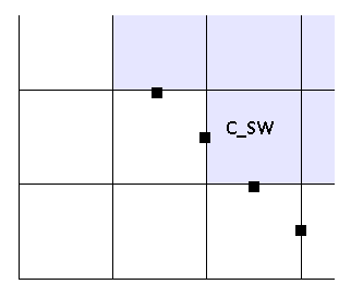
          case GG.C_SW:
            {
              U[i][j - 1] = U[i][j];
              V[i][j - 1] = V[i][j];
              U[i - 1][j] = U[i][j];
              V[i - 1][j] = V[i][j];
            } break;
Here we do not need the values in the cell itself - they will be calculated in the solver. But then we need values in neighboring empty cells - because in the solver there are terms with U [i] [j - 1], etc.
The nearest water cell to these empty cells is the cell [i] [j] from it and the values U and V are taken.
From the figure it can be seen that the value for V [i - 1] [j] could be taken as from cell [i ] [j], as well as from [i - 1] [j + 1] - but in the general case the cell [i - 1] [j + 1] may turn out to be non-water, and the value of V in it may also turn out to be boundary and will not be affixed yet. Therefore, the correct option is [i] [j] because the values in it will be calculated in the solver.
flag cage C_W
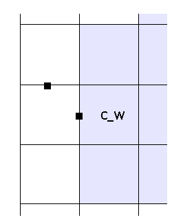
          case GG.C_W:
            {
              U[i - 1][j] = U[i][j];
              V[i - 1][j] = V[i][j];
            } break;
Everything is similar here.
cell with flag C_NW
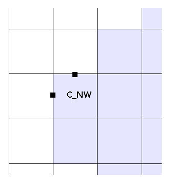
          case GG.C_NW:
            {
              V[i][j] = V[i][j - 1];
              U[i - 1][j] = U[i][j];
            } break;
Here, the value of U in the cell itself will be calculated in the solver, because there is a water cell to her right. But V needs to be put down, since the cell above is empty. It is also necessary to set the value U [i - 1] [j], since when calculating U [i] [j], values will also be required in the cells adjacent to it, including in U [i - 1] [j].
In the same way as in the previous case, we take the value V [i] [j] from the cell V [i] [j - 1], and not from V [i-1] [j] - the value in V [i-1 ] [j] may turn out to be boundary and not yet known.
We set the pressure in empty cells and surface cells = 0. This is not entirely correct, but it works.
In surface cells, pressure is necessary, because when solving the equation for pressure, these cells are boundary and pressure calculation is not performed directly in them.
Particle-only fluid motion algorithm
In the source there are options with the name track in the title. This is a method of moving a free surface in which particles move only on the surface itself, and not in the entire volume of the liquid. This is somewhat similar to the VOF method - but preliminary reconstruction of the surface is done there, which is rather cumbersome. In my method, if a particle leaves a cell, it is marked empty, and particles are added to nearby liquid cells in which there are no particles - to know where the surface is. If the particle passes into an empty cell, then the cell is marked as liquid. Of course, this method has a decent share of inaccuracy, but it is fast and does not require complex coding.
Implicit calculation scheme
There is also an implicit version of the solver in the sources - it is applied to equations for speeds, the differences in the code from the explicit version are minimal there. When sampling, simply all terms with U and V [i] [j] go to the left side of the equation and not to the right as in explicit.Implicit (implicit) scheme allows you to take significantly larger time steps, which is impossible with explicit.
You can read about implicit here http://math.mit.edu/cse/codes/mit18086_navierstokes.pdf .
3D version
In the 3D version, everything is done by analogy with 2D.
Controls F1-F8 + WASD keys, arrows and ER PgUp PgDown to rotate the camera.
For scenes with a water source - P key - to turn off the water pressure.
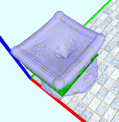
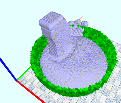
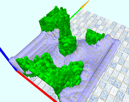
G - better surface rendering (spheres are used instead of cubes), but it terribly slows down.
In the Demos folder - there are scenes and parameters (sizes, time step, gravity and number of particles per cell) in the form of an xml file. It is also possible to paint your HeightMap (map of heights) in paint, sizes can be any - there are autoresize.
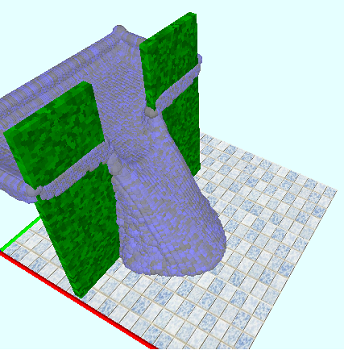
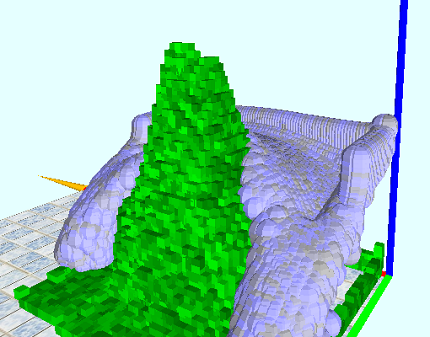
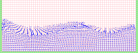
In conclusion, I will give screenshots from 2D and 3D:
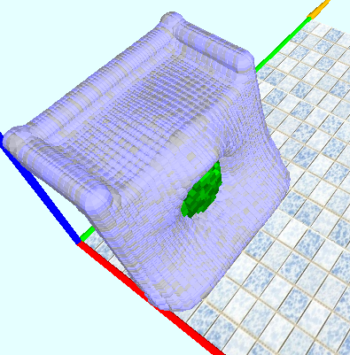
The rest of the screenshots here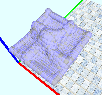
Sources are here sourceforge .
Projects that are in the source
Все написано на Visual Studio 2010
— Adaptive Mesh Refinement — клетки разбиваются на более мелкие части и в этих дочерних ячейках тоже считаются
все переменные, при этом крупные клетки являются соседними к дочерним при дискритизации
fluid2subcell*
— implicit версия
fluide2dimplicit\ и fluide2dimplicitfree\
— программа разбита на модули, которые легко заменять на другие версии, не удаляя старые
fluide2dmodule\
— движение воды реализовано через движение частиц только на поверхности
fluide2dtrack*
— рабочая версия с explicit методом и граничными условиями на поверхности, которые описаны в данном посте
simpletestobstacle\
— вместо безразмерного Re — используются реальные коэффициенты плотности воды и вязкости ,
что позволяет при решении уравнений сразу получать настоящие скорости и реальное давление в массивах U V P
simpletestobstaclereal\
— все что есть в папке finite volume относится к этому методу
сделано по книге:
Introduction to computational fluid dynamics The finite volume method Versteeg HK Malalasek
— теперь 3D
— простейший вариант — без поверхности и препятствий
SimpleFluid3D\
— самый последний вариант со всем всем всем на с++
fluid3dunion\
— вариант для GPU ( только вода ), написан на OpenCL, на моей GeForce 550 ускорение в 7 раз (без каких либо оптимизаций специально под gpu)
fluid3clsimple\
— очень ранняя версия того что есть в fluid3dunion — версия рабочая, но есть много недоработок, на c#, explicit
fluide3tao
Ссылки по теме
Хорошая статья есть тут Kalland_Master.pdf
и тут Кратко о гидродинамике: уравнения движения
Книги:
— Griebel M Dornseifer T Numerical simulation in fluid dynamics SIAM 1998
// эту книгу особенно отмечу, с нее фактически все началось у меня, исходники к ней легко можно найти, лучшего описания реализации cfd я до сих пор не нашел)
— Bridson R. Fluid Simulation for Computer Graphics
— Anderson JDJr Computational fluid dynamics The basics with applications MGH 1995
— Charles Hirsch-Numerical Computation of Internal and External Flows 2007
— Gretar Tryggvason Direct Numerical Simulations of Gas-Liquid Multiphase Flows
- Versteeg HK Malalasek Introduction to computational fluid dynamics The finite volume method
All books can be found yourself know where.
PS If there are people familiar with CFD, it would be interesting to improve this project together in terms of speed and correctness of the solution (especially when modeling the surface).
I myself can render rendering more or less, but mathematics and physics are not my main area. I will be glad to any comments and useful tips.